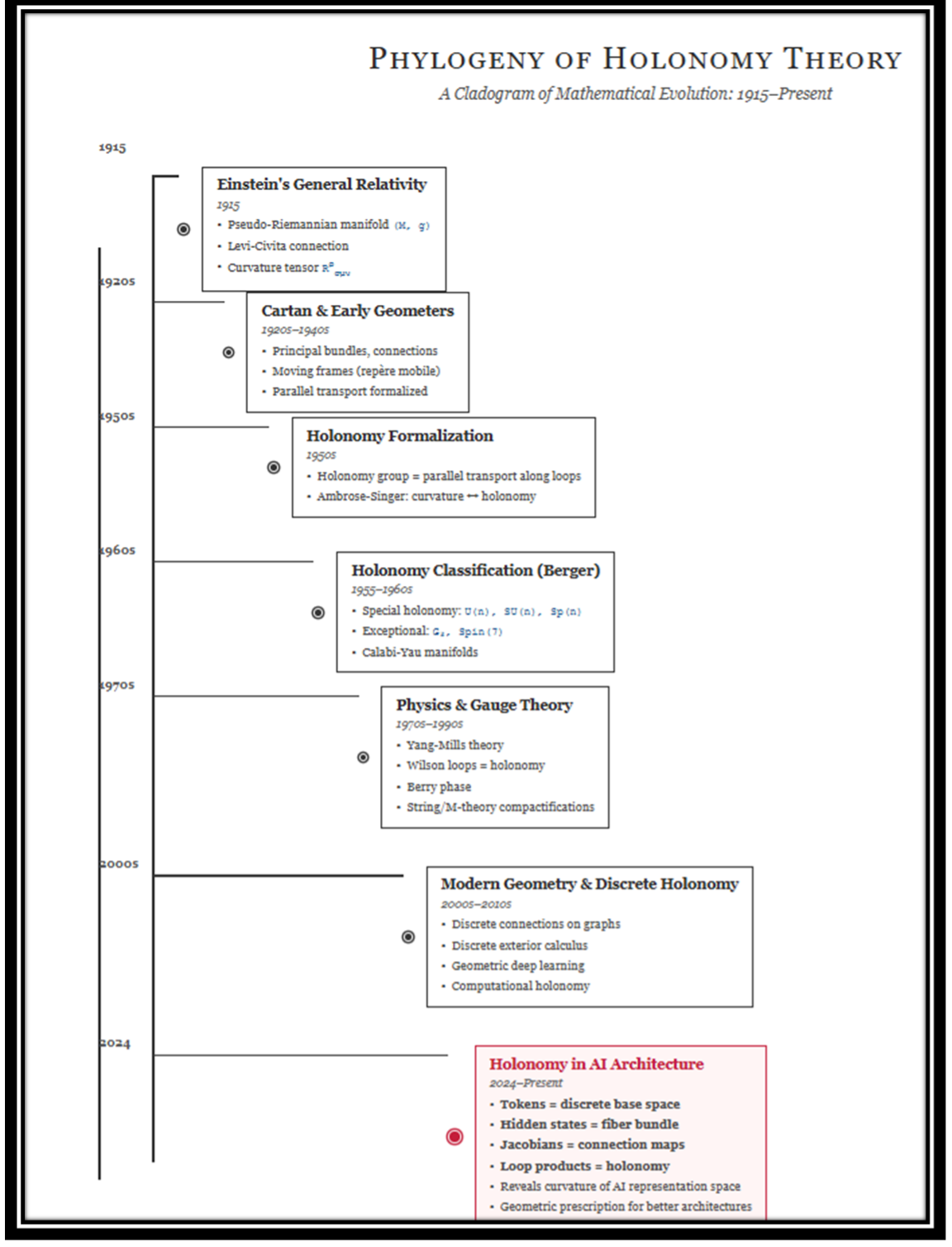
Holonomy, From Einstein to Deep Learning

Born in Einstein’s geometry of gravity, holonomy now gives us the language to measure curvature in neural networks and explain why flat Euclidean AI keeps breaking.

The evolution tree of holonomy theory: from Einstein to modern AI

Let’s take this slowly.

Holonomy sounds like a word only a geometer could love.
But the idea is very simple:

Move a vector around a loop.
If it comes back twisted, the world is curved.

That’s it.
Everything in your cladogram is just this idea getting sharper, cleaner, more abstract — until it finally lands in our neural networks.

We’ll walk the tree together.

1. Einstein’s Curved Spacetime (1915)

Start at the root.

Einstein takes spacetime and says: it’s not a stage, it’s a field.
Mathematically:

\(\begin{array}{l} \text{• a (pseudo-)Riemannian manifold } (M, g), \\ \text{• with a metric } g_{\mu\nu} \text{ telling you lengths, times, light cones.} \end{array}\)

\(\begin{array}{l} \text{To make physics work, you need a way to "compare" vectors at different points.} \\ \text{Enter the } \textbf{Levi--Civita connection } \nabla, \text{ packaged in the Christoffel symbols } \Gamma_{\mu\nu}^\rho. \\ \\ \text{You pick a vector at some event in spacetime.} \\ \text{You } \textbf{parallel--transport} \text{ it along a curve using these } \Gamma_{\mu\nu}^\rho. \\ \\ \text{Now the key: derivatives don't commute.} \\ \text{The } \textbf{curvature tensor } R_{\sigma\mu\nu}^\rho \text{ measures exactly how much "go this way} \\ \text{then that way" differs from "that way then this way."} \end{array}\)

Einstein is already living in a world where:

• paths matter,

• loops encode information,

• curvature is physical (gravity).

He doesn’t say holonomy group yet. But the seed is there:
vectors carried around loops don’t come back the same.

---

2. Cartan and the Upgrade to Bundles

Now geometers get hungry.

Einstein works mostly in coordinates. Cartan comes and says:
forget coordinates; use frames and bundles.

• Take your manifold M.

• Over every point, attach a little frame — a basis for tangent space.

• Collect all these frames: you get a principal bundle P→MP

A connection is now an object on this bundle telling you how to move frames along curves. You can still ask:

If I move a frame around a loop and come back, how is it rotated?

That rotation is no longer just an accident; it’s a structural feature of the connection.

Cartan’s move matters for us because this is exactly what we’ll do in AI:

• base = tokens / sites,

• fibers = representation spaces,

• connection = Jacobian transport.

He gave us the language for AI!

---

3. Holonomy Gets a Name

Next step in the cladogram: people stop hand–waving and give the loop-effect a precise identity.

Given:

• a bundle P→M with structure group G,

• a connection on it,

you fix a point p ∈ P and look at all loops in M based at its projection.

Each loop gives you a group element in G — “how the frame changed after going around.”
All those elements together form the holonomy group at that point.

This is holonomy in the modern sense:

Holonomy = the group generated by all parallel–transport maps around all loops based at a point.

Then Ambrose–Singer come in and show a beautiful fact:

• local: curvature tensor and its covariant derivatives

• global: holonomy group

are tightly linked.

The holonomy group is basically the global shadow cast by curvature.

This is the same logic we’ll apply to networks in AI:

• local data: Jacobians between sites,

• global data: products of Jacobians around loops.

If the loop map is not identity, the representation geometry is curved.

---

4. Berger and the Zoo of Holonomy Groups

Now that holonomy is a first–class citizen, geometers ask:

“What holonomy groups are actually possible?”

Berger answers with a classification:

• Generic Riemannian manifolds: holonomy SO(n).

• Special structures: Kähler, Calabi–Yau, hyperkähler, G₂, Spin(7) — each with their own holonomy subgroup.

Holonomy now does two things:

1. It detects curvature (Einstein’s game).

2. It classifies geometry (Berger’s game).

You look at the holonomy group and immediately know what kind of extra structure the manifold carries: complex, symplectic, exceptional, …

File this pattern away.
We’ll steal it for AI: holonomy as both detector and classifier of network geometry.

---

5. Physics and Gauge Theory: Loops Become Observables

Then physics returns.

Gauge theory reuses the same bundle–connection–holonomy package, but now the structure group is something like SU(2) or SU(3).

A gauge field is a connection.
A Wilson loop is the holonomy of that connection around a closed spacetime loop.

You can read it as:

“How much does the internal state of a particle rotate if I drag it around this loop in the gauge field?”

That rotation is measurable.
Holonomy stops being just a geometric curiosity and becomes a physical observable.

Again, the pattern we like:

• local: gauge potential and curvature,

• global: holonomy around loops,

• meaning: whether the field configuration is trivial or stores real, physical structure.

---

6. Modern & Discrete Holonomy

Fast–forward.

Geometry spreads into computation:

• Discrete differential geometry puts connections on meshes and graphs.

• You parallel–transport vectors along edges.

• You take products along cycles.

• Holonomy appears in graphics, shape analysis, geometric deep learning.

The space may be combinatorial, but the idea is identical:

edges = tiny transports,
cycles = loops,
holonomy = what you see after one tour.

We’re almost home.

7. Holonomy in AI: Jacobians as a Connection

Now we step into the red box of our cladogram above: Holonomy in AI Architecture.

\(\begin{array}{l} \text{Stop. Look at your network as a geometer would.} \\ \\ \text{• Base } B\text{: sites --- tokens, patches, slots, positions.} \\ \text{• For each site } i, \text{ a fiber } V_i \simeq \mathbb{R}^d\text{: the local representation space.} \\ \quad \text{One fiber, one token.} \\ \\ \text{Collect all fibers: you get a vector bundle } E = \coprod_{i \in B} V_i \to B. \\ \text{A full layer state is a point in the product } \prod_{i \in B} V_i. \\ \\ \text{Now apply automatic differentiation.} \\ \\ \text{For a block } F, \text{ the Jacobian block} \\ \\ J_{ij} = \frac{\partial y_j}{\partial x_i} \\ \\ \text{tells you how a tiny tweak at site } i \text{ shows up at site } j \text{ after the block.} \\ \\ \text{Geometrically, that's a linear map} \\ \\ \Gamma_{ij} : V_i \to V_j. \end{array}\)

This is no longer “just a derivative.”
It’s a transport operator between fibers.

All these Γij​ together form a discrete GL(d)-connection on your representation bundle.

Now you can play the Einstein–Cartan–Ambrose–Singer game inside the network.

Pick a loop of sites:

i→j→k→i

Compose the transport maps:

\(H_{ijk} = \Gamma_{ki} \, \Gamma_{jk} \, \Gamma_{ij} : V_i \to V_i.\)

This is your holonomy operator for that loop.

\(\begin{array}{l} \text{• If } H_{ijk} = I \text{ for all loops, your connection is flat: the representation space} \\ \quad \text{behaves Euclidean.} \\ \text{• If some } H_{ijk} \neq I, \text{ you've detected } \textbf{curvature} \text{ in how the model moves} \\ \quad \text{information around.} \end{array}\)

You didn’t add any fancy manifold.
You didn’t force the model to live in hyperbolic space.
You just looked at what its own Jacobians are already doing.

The code pretends to live in flat R^n,
but the holonomy of its Jacobians exposes a curved, path–dependent geometry underneath.

That’s the punchline.

---

8. Why This Matters for “Flat AI”

Modern deep learning still reasons in a flat Euclidean mindset:

• tensors in R^n,

• gradients as simple vectors,

• loss landscapes sketched as nice bowls.

But the actual behavior of perturbations inside a large model is path–dependent, anisotropic, and often wildly tangled.

Holonomy gives you a language for this:

• Fibers: where representations live.

• Connection (Jacobians): how a nudge at one site becomes a nudge elsewhere.

• Loops: how information flows around motifs in the architecture.

• Holonomy: the net twist you get after a tour — the fingerprint of curvature.

Once you adopt this lens, “model failure” stops being purely a stochastic or optimization story and becomes a geometric one:

• exploding / vanishing directions,

• brittle generalization,

• weird trajectory dependence,

are all hints that the connection is badly behaved — too much curvature in the wrong places, or curvature aligned with the wrong subspaces.

---

Conclusions: From Einstein’s Spacetime to Our Transformer AI

If you zoom out, your cladogram reads like one continuous thought:

1. Einstein: curvature is physical, paths matter.

2. Cartan: connections and bundles are the right language.

3. Ambrose–Singer: curvature and holonomy are two sides of the same coin.

4. Berger & physics: holonomy classifies and explains real structure.

5. Discrete geometry: we can do this on graphs.

6. Deep learning: our models are graphs with Jacobians on the edges.

So the move is natural:

Treat a neural network as a discrete geometric object,
read its Jacobians as a connection,
compute holonomy along loops,
and let curvature tell you where the architecture is secretly twisted.

Einstein used this logic to understand gravity.
We can use the same logic to understand why flat Euclidean AI keeps breaking, and how to build architectures whose geometry actually matches the problems they’re meant to solve.

That is the real message of our diagram:
holonomy didn’t stop in spacetime physics.
It now has a new habitat — the hidden geometry of neural networks.