

Rethinking Network Strategies: Where Most AI Data Centers Miss the Mark
Exposing the Oversights in AI Infrastructure's Connectivity and Efficiency


In the race to build powerful AI systems, simply accumulating more hardware-GPUs and CPUs-is not enough. It seems, as the big IT moguls suggest while announcing massive layoffs, that there’s no need to rely on engineers who will soon be replaced by smart data centers armed with the latest AI models; just keep purchasing more GPUs than the competition. However, this approach misses a crucial point: the key to truly efficient AI data centers lies in the careful design of their topology and network architecture. Without proper planning, even the most resource-rich setups will inevitably lead to perpetual traffic congestion.
Rethinking Traditional Topologies in AI-Oriented Data Centers
It’s a misconception that hardware alone can drive advancements; the expertise of engineers in system design and optimization remains irreplaceable. Engineers play a crucial role in ensuring that AI infrastructure is not only large but also smart and efficient, highlighting the importance of thoughtful design over mere scale.
Traditional topologies like Point-to-Point, Leaf-Spine, and Three-Layer networks, each with its distinct architecture and operational dynamics, have served as the backbone of data center design.
However, as AI workloads grow in complexity and demand, these traditional frameworks show clear shortcomings. Initially cost-effective, these topologies quickly reveal their limitations as data centers scale up to support more demanding AI models. The degradation in performance soon jeopardizes the viability of the entire project, underscoring the urgent need for network architectures that can efficiently accommodate the rapid expansion and intensive computational requirements of advanced AI systems.
Let’s revise the cases in point:
Point-to-Point Topology: the topology’s poor man
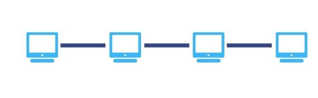
If there’s one certainty in the realm of AI model development, it’s the universal recognition among GPU users of this topology’s inadequacy. The digital world’s answer to the frugal man’s networking: a scenario where every device demands its own direct line, like an old-fashioned party line where everyone’s connected but in the least efficient way possible. It’s akin to using carrier pigeons for your daily emails; comically impractical, turning your data center into a digital traffic jam.
Anyway for educational purposes let’s examine the miserable conditions of complexity and scaling this topology is dealing with:
Complexity : In a point-to-point topology, every device must be directly connected to every other device for direct communication. If N represents the number of GPUs, then the number of connections ( C ) needed can be approximated by the formula C=N(N−1)/2 C = N ( N −1)/2. This is because each GPU needs a connection to every other GPU, but this count includes each connection twice (A to B, and B to A), hence the division by 2.
Doubling GPUs : When the number of GPUs doubles (2 N ), the number of connections becomes 2 N (2 N −1)/2, which simplifies to N (2 N −1), showing a quadratic increase in connections.
Leaf-Spine Topology
Stepping up from the digital quagmire of point-to-point, the leaf-spine topology emerges as the middle child of network configurations. Picture it as the more refined sibling, moving from the chaotic approach where each device connects directly to others, to a structured system.
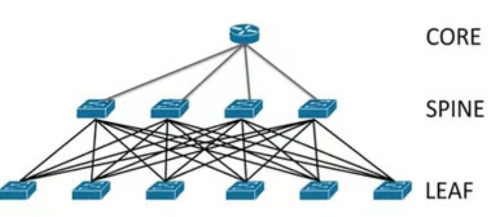
Each leaf (switch) connects to every spine (switch), creating pathways more akin to a well-planned subway system than the P2P tangled mess of city streets. While it marks a leap towards efficiency, leaf-spine still lags behind the hypercube’s elegance, like trading in a horse and buggy for a car when you could be flying a jet.
Complexity : The leaf-spine topology is designed to reduce the complexity of point-to-point connections by using a set number of spine switches to interconnect leaf switches, to which GPUs are connected. While this reduces direct connections, the complexity increases linearly with the number of leaf switches and the number of spine switches needed grows as the network expands. Mathematically C primarily depends on the number of leaf switches ( L ) and the number of spine switches ( S ). Each leaf switch is connected to every spine switch to ensure high availability and fault tolerance, leading to a total connection count of: C = L × S . If each leaf switch supports G GPUs, and the total number of GPUs in the system is N , then: L = GN , assuming each leaf switch needs to connect to each spine switch for full connectivity, the complexity increases linearly with the number of GPUs as they dictate the number of leaf switches required.
Doubling GPUs : Assuming each leaf switch supports a fixed number of GPUs, doubling the GPUs would require doubling the leaf switches. The spine switches might also need to increase to maintain optimal performance, leading to a linear (but substantial) increase in complexity and cost. Mathematically: Doubling the number of GPUs (2 N ) would theoretically double the number of leaf switches (2 L ) required if each switch supports a fixed number of GPUs ( G ). This might not necessarily double the number of spine switches, but to maintain performance and avoid bottlenecks, an increase in spine capacity or number could be necessary, implying:adjusted_ C_ new=2 L × S_ adjusted
Three-Layer Topology
This traditional structure, with its distinct core, distribution, and access layers, is less flexible and performant compared to the leaf-spine model. Let’s explore the reasons why:
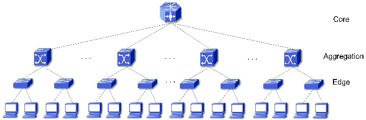
Complexity Let’s denote the number of core switches as ©, distribution switches as (D), and access switches as (A). The total complexity can be considered as the sum of connections between these layers, which also involves the management and operational overhead. As the number of GPUs increases, requiring more access switches (A), this might necessitate additional distribution switches (D) to manage increased traffic, and potentially more core switches © for higher throughput, leading to a non-linear increase in complexity due to the hierarchical nature: Complexity approx = A + D + C
Doubling GPUs necessitates a reevaluation of each layer’s capacity. More access switches (2A) are needed, possibly requiring more distribution switches to handle the increased load (D), and potentially more core switches for interconnectivity ©. This results in: 2A + D + C The precise impact on (D) and © depends on the existing topology’s design and the incremental capacity of each layer. Unlike the hypercube topology, where complexity grows logarithmically with the addition of nodes, both Leaf-Spine and Three-Layer topologies exhibit linear or potentially super-linear growth in complexity and associated costs as the network scales , primarily due to the increased number of switches and connections required to maintain system integrity and performance.
Hypercube Topology: A Superior Alternative
And now, our rocky star. Let’s delve into its almost magical properties.
Understanding the Hypercube Topology
- Logarithmic Scaling Efficiency : In contrast, the hypercube topology presents an elegant solution to these scalability issues. Its design allows for connectivity to expand logarithmically rather than linearly with the addition of nodes. Each new dimension in the hypercube doubles the number of nodes, enhancing the network’s capacity without proportionally increasing its complexity or cost. This means that for a hypercube of dimension (D), adding another dimension creates a network that efficiently integrates twice as many GPUs while maintaining optimal path lengths and minimal increase in connection complexity. Mathematically the number of nodes N is determined by 2^ d , where d is the dimension of the hypercube. This means that each increase in dimension doubles the number of nodes. For instance, adding a dimension to a 3-dimensional cube (8 nodes) transforms it into a 4-dimensional hypercube with 16 nodes. However, despite the exponential growth in nodes, the complexity of communication-or the number of steps required for any node to communicate with another-only increases logarithmically, log2(N) . This property is what sets the hypercube apart from more traditional topologies.
Yeah, cool, but what can I do if I have already screwed up my network and can’t rewire to a hypercube?
If your legacy network is a leaf-spine architecture, then, dear tech bro, you’re in luck. Among the three previously mentioned topologies, the leaf-spine architecture stands out as the prime candidate for a hybrid scale-up approach. By simply programming with MPI, your graph can map smoothly through your software to a hypercube, retaining the most crucial properties as if you had done it via hardware.
Otherwise, applying MPI to convert a three-layer architecture into a hypercube involves significant challenges due to the hierarchical nature of the three-layer setup. While MPI can facilitate communication between nodes in a distributed system, the rigid separation of core, distribution, and access layers in a three-layer architecture may limit the effectiveness of this approach. Anyway , dont lose hope, it is still a way to overcome the challenges with MPI and C: you can start by mapping your network’s physical topology to a logical hypercube structure in software. Using MPI, you can create groups and communicators that reflect this hypercube layout, allowing for efficient parallel communication patterns. Within your C code, you’d use MPI functions to manage data exchange between nodes, employing algorithms that take advantage of the hypercube’s properties, like reduced communication steps. Of course this requires a deep understanding of both your network’s current architecture and MPI’s capabilities to create a layer that abstracts the physical topology into a more efficient, hypercube-like logical structure.
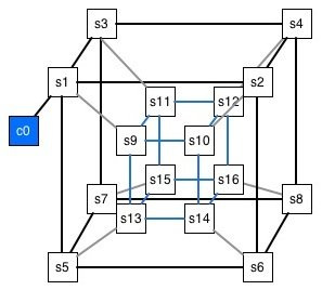
Implementing a hybrid programmatic solution with MPI and C to optimize your network towards a hypercube-like topology will result in a structured graph representation of your network’s nodes and connections. This graphical model, as illustrated inFigure 5, visually demonstrates the steps in accessing the other nodes. It showcases the logical arrangement of nodes and the efficient pathways established between them, highlighting the improved communication flow and reduced complexity achieved through the application of our hybrid solution.
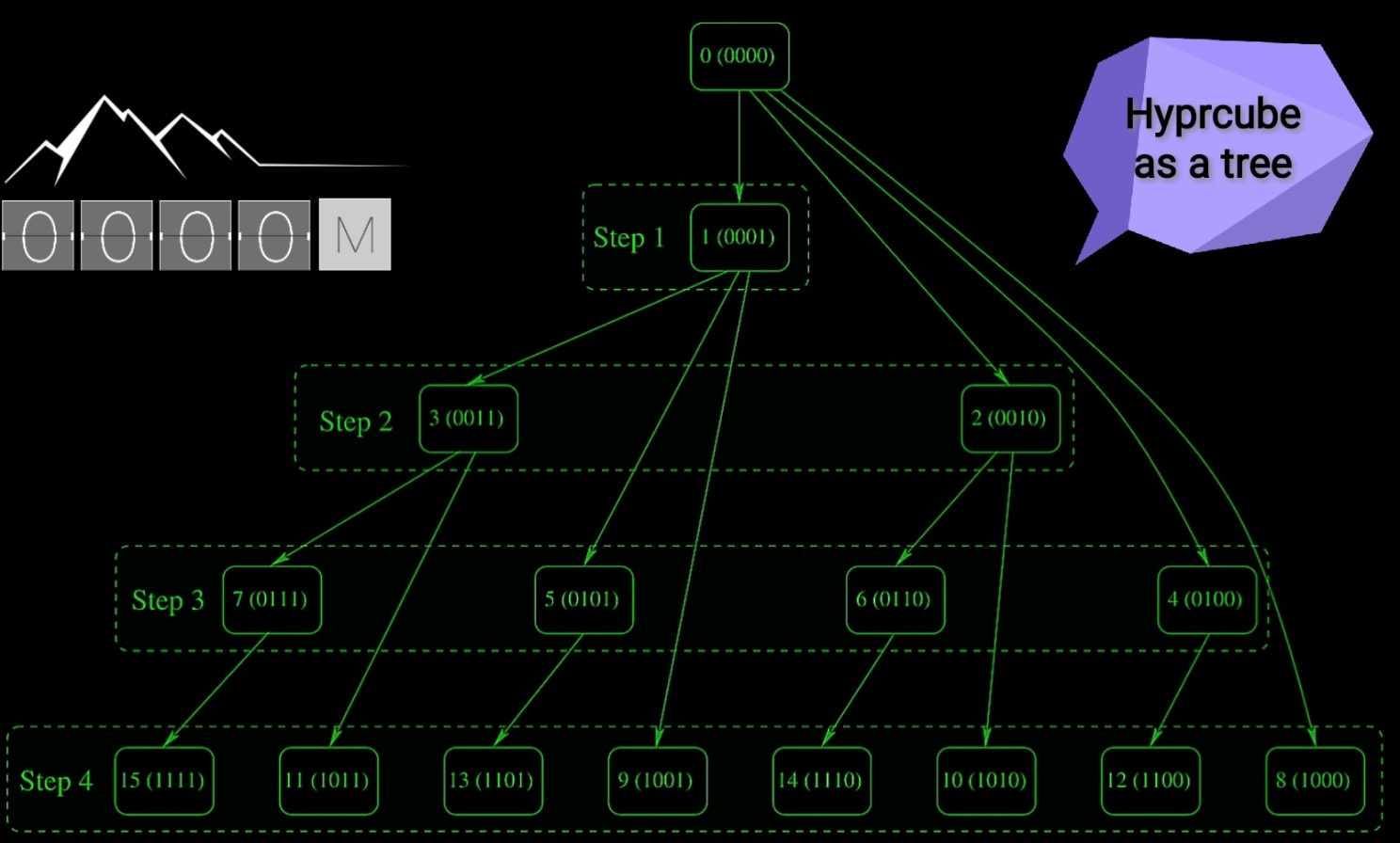
In fact the fig 5. illustrates how a message is broadcasted in a hypercube structure according to the SW with MPI. The nodes are labeled with both their rank and their corresponding binary representation. The illustration shows the progressive steps of the message broadcasting:
Step 1: The node with rank 0 (0000 in binary) sends the message to node 1 (0001 in binary).
Step 2: Node 1 then sends the message to node 3 (0011 in binary), while node 0 sends to node 2 (0010 in binary).
Step 3: The broadcasting continues with nodes 2 and 3 sending messages to nodes 6 (0110 in binary) and 7 (0111 in binary), respectively, and node 1 sending to node 5 (0101 in binary), and so on.
Step 4: This step would show further broadcasting to higher-ranked nodes as the message propagates through the hypercube structure.
Each line connecting the nodes represents the communication link over which the message is sent. The figure indicates the dimensions of the hypercube that are being used for communication at each step, demonstrating the hypercube broadcast algorithm’s property: here lies the hypercube’s magic. While the number of nodes grows exponentially, the path length — or the maximum number of steps from one node to another — increases only logarithmically with the number of nodes. This means that even as the network grows, the efficiency of communication between any two GPUs remains incredibly high.
AND NOW MONEY, MONEY, MONEY…
Crunching the Numbers: The Cost of Tradition vs. The Hypercube Advantage
Let’s talk dollars and sense. Considering the initial setup cost for a data center network designed to support 1000 GPUs, traditional topologies like leaf-spine and three-layer architectures could cost over $700K . It seems reasonable until realizing that expanding to accommodate another 1000 GPUs could inflate operational costs to around $3 million annually — a financial misstep akin to watering a garden with a fire hose: wasteful and problematic.
But here’s the twist: expanding the network with our hybrid model to support an extra 1000 GPUs would only increase annual operational costs by slightly over $200K, not $3 million. This isn’t just saving; it’s a paradigm shift in scaling AI infrastructure, offering not just a lifeline but a jetpack for managing AI’s exponential growth.
In an upcoming article, I will show how this hybrid model can be implemented in two flavors: with C and MPI, and C++ 20 with an improved version of MPI. Stay tuned.