

The Missing Mathematics of AI
The poor insufficient math foundations of our commercial AI stacks

The Missing Mathematics of AI
Why Commercial AI Stacks Are Built on Incomplete Foundations
Jose Crespo, PhD
Modern AI frameworks—PyTorch, TensorFlow, JAX, and the ecosystem built upon them—implement a remarkably narrow slice of the mathematics available for learning systems. This article presents a rigorous analysis of the mathematical domains that govern inverse problems and identifies the specific gaps in commercial implementations. We argue that these omissions are not accidental but reflect deep structural blind spots in how the field conceptualizes machine learning. The consequences range from unexplained training instabilities to fundamental limitations in what current architectures can reliably learn.
1. The Taxonomic Position of Machine Learning
Before analyzing what commercial stacks lack, we must establish where machine learning sits within mathematics. This positioning is not merely academic: it determines which mathematical tools are appropriate and which pathologies are inevitable.
1.1 Machine Learning as Inverse Problem
Every supervised learning task has the same formal structure. Given observations y = F(θ, x) + ε, we seek parameters θ that explain the data. This is precisely the definition of an inverse problem: given the output of an operator, recover its input or parameters.
Jacques Hadamard formalized in 1923 the conditions under which such problems are well-posed: existence of a solution, uniqueness of that solution, and continuous dependence on the data. Virtually no machine learning problem satisfies all three conditions. Neural networks are overparameterized (non-unique solutions), loss landscapes have spurious minima (existence issues for global optima), and small perturbations to training data can produce radically different models (discontinuous dependence).
This classification has immediate consequences. Inverse problems require regularization: additional constraints that make the problem tractable. The entire history of successful regularization theory, from Tikhonov to total variation to Bayesian priors, applies directly to machine learning. Yet commercial stacks implement almost none of it.
1.2 The Hierarchical Structure of Relevant Mathematics
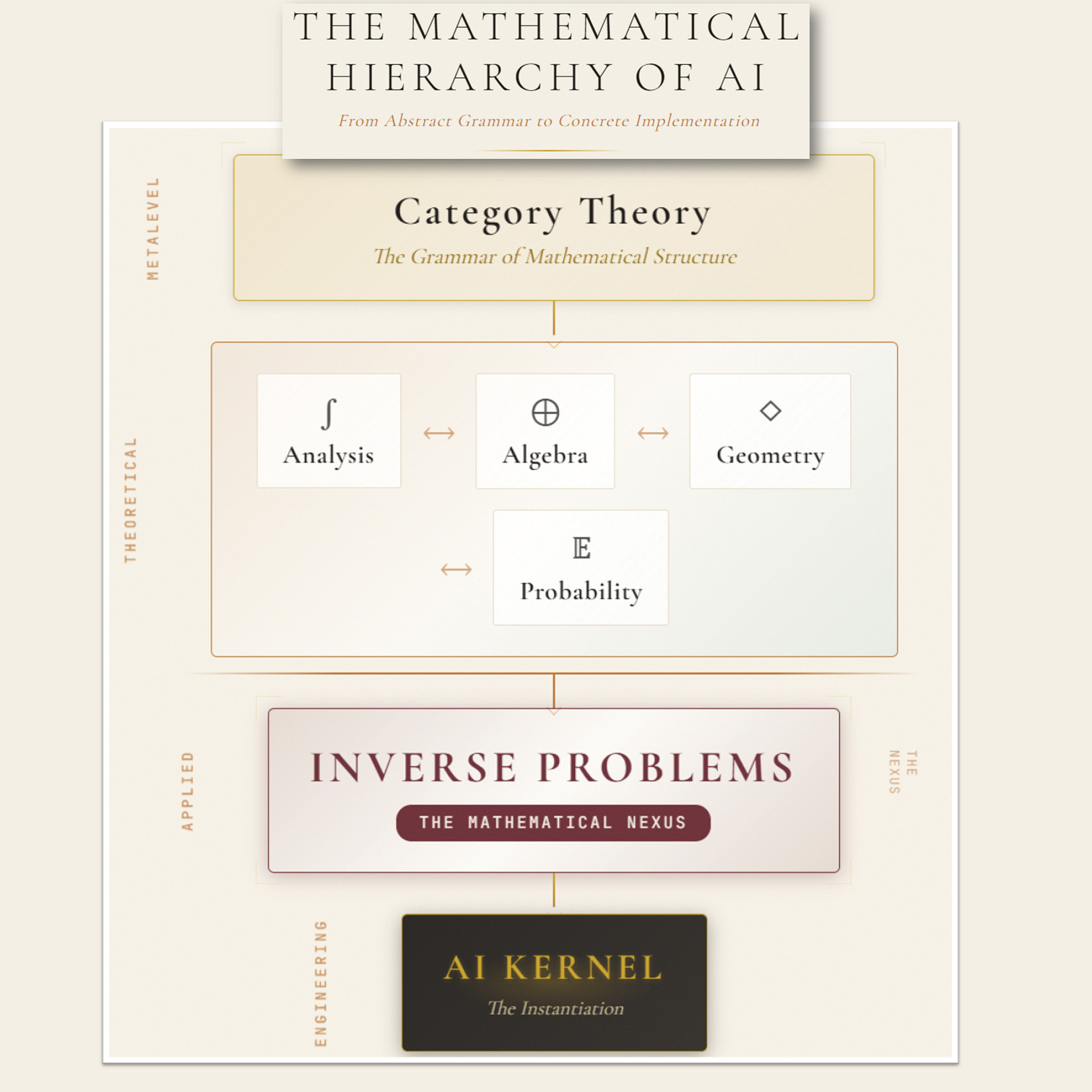
Inverse problems sit at the intersection of multiple mathematical domains, each contributing essential structure:
Functional Analysis provides the framework for operators between infinite-dimensional spaces. Neural networks are approximations to such operators, and their properties—compactness, spectral decay, continuity—determine trainability.
Operator Theory characterizes forward and inverse maps through their spectra. The singular value decomposition of linear operators generalizes to neural networks as the spectrum of the input-output Jacobian. Ill-conditioning manifests as clustered or decaying singular values.
Differential Geometry describes the intrinsic structure of parameter spaces. Weight matrices often lie on manifolds (orthogonal groups, positive definite cones), and ignoring this structure forces optimization through unnecessarily difficult terrain.
Category Theory provides the metalanguage for compositional structure. Forward operators are functors; inverse operators are adjoints. Composition of layers must respect diagram commutativity to preserve semantic meaning.
Group Theory determines identifiability through symmetry analysis. Weight space symmetries (permutation invariance, scaling) create equivalence classes; learning should optimize over quotient spaces, not raw parameters.
Probability Theory (Bayesian formulation) recasts regularization as prior specification. Every regularizer corresponds to a prior distribution; L2 regularization is a Gaussian prior, L1 is Laplacian, and geometric regularizers encode structured beliefs about parameter relationships.
2. Spectral Theory: The Invisible Scaffold
The most consequential omission in commercial AI stacks is spectral analysis. Every claim about generalization, stability, and trainability ultimately reduces to spectral properties of operators derived from the network architecture and data.
2.1 The Hessian Spectrum and Generalization
Consider the loss function L(θ) as a functional on parameter space. Its second derivative, the Hessian H = ∇²L, encodes complete local curvature information. The spectrum of H—its eigenvalues {λᵢ}—determines fundamental properties of training dynamics and learned solutions.
What Eigenvalues Reveal
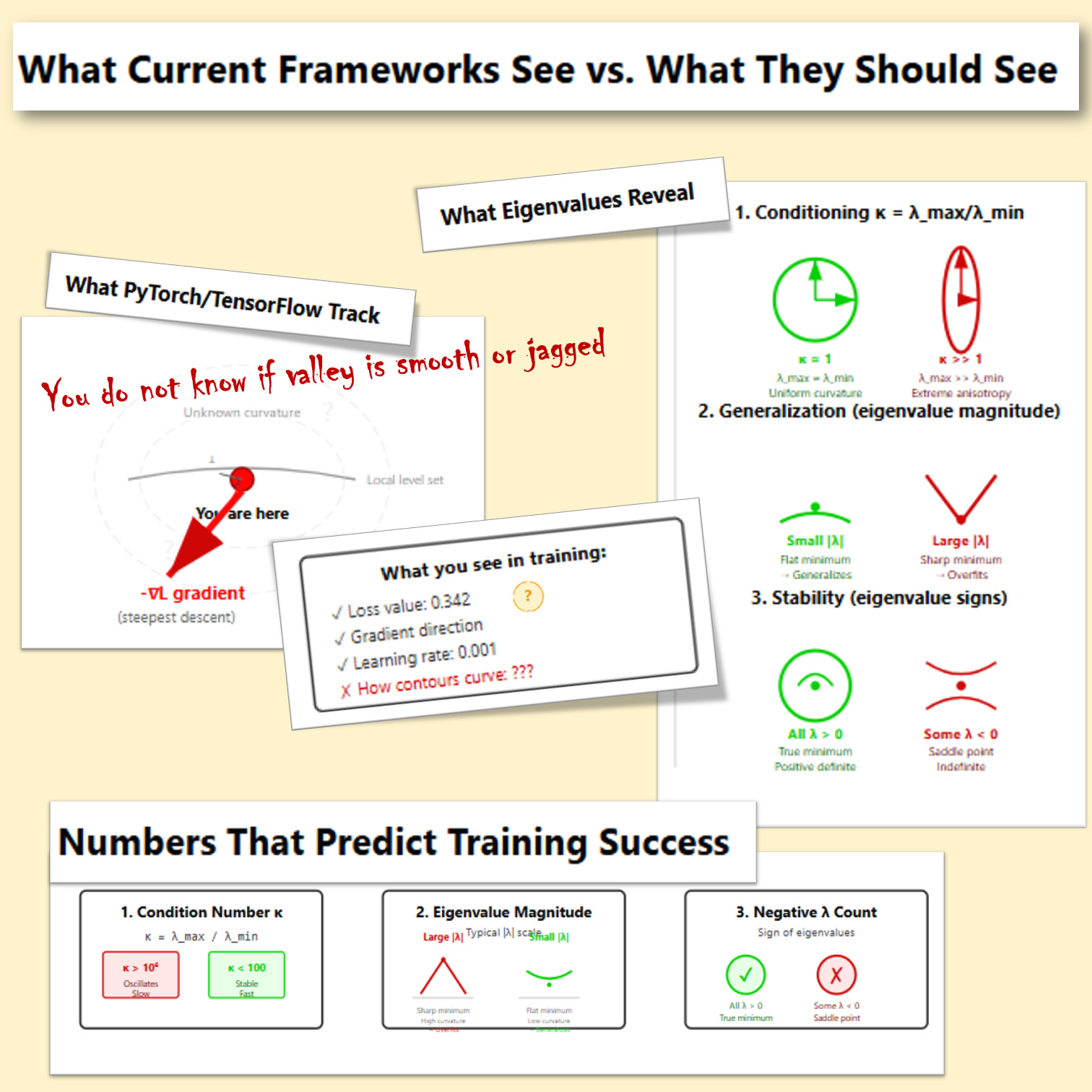
Condition Number and Training Stability. The condition number κ = λₘₐₓ/λₘᵢₙ is the canonical measure of optimization difficulty. For gradient descent, the convergence rate scales as (κ−1)/(κ+1) per iteration. High κ means the loss landscape is “elongated”—steep in some directions, flat in others—forcing zigzag trajectories that waste computational effort.
This is not merely theoretical. The edge of stability phenomenon, empirically documented across architectures, confirms that gradient descent naturally finds and hovers at λₘₐₓ ≈ 2/η (where η is the learning rate). The optimizer self-organizes to the boundary of stability defined by the largest eigenvalue.
Important caveat: In practice, κ can be astronomically large (10¹⁴ or more in some studies), yet training still succeeds. This apparent paradox resolves because SGD noise effectively “regularizes” the spectrum: stochasticity helps escape ill-conditioned directions. The condition number constraint applies most strictly to full-batch gradient descent; mini-batch SGD operates under a softer regime.
Eigenvalue Distribution and Minimum Geometry. The bulk of the Hessian spectrum characterizes the geometry of the solution. Empirical studies (Sagun et al., 2016; Ghorbani et al., 2019) reveal a consistent bulk + outliers structure: most eigenvalues cluster near zero, with a few large positive outliers.
Many small eigenvalues indicate a flat minimum—low curvature in most directions means the loss surface resembles a plateau rather than a sharp valley. Such minima tend to be stable under parameter perturbation and correlate empirically with better generalization.
Many large eigenvalues indicate a sharp minimum, high curvature means small parameter changes produce large loss changes. Such minima correlate with poorer generalization, though the causal mechanism remains debated.
Theoretical nuance: The flatness-generalization connection is empirically robust but theoretically contested. Dinh et al. (2017) demonstrated that reparametrization can change eigenvalues without changing the function: a “sharp” minimum can be made “flat” by rescaling weights. The principled justification comes through PAC-Bayes bounds: small eigenvalues mean the loss changes little under parameter perturbation, yielding tighter generalization bounds. The correlation is real; the mechanism is subtle.
Negative Eigenvalues and Saddle Points. At any critical point (where ∇L = 0), eigenvalue signs classify the point’s nature (See Figure 2 above):
All positive → local minimum
All negative → local maximum
Mixed signs → saddle point
In high-dimensional spaces, saddle points dominate overwhelmingly. A simple Bernoulli argument suggests the probability of a true minimum (all eigenvalues positive) decreases exponentially with parameter count. For networks with millions of parameters, essentially all critical points are saddle points:which is actually good news, since saddle points are dynamically unstable and SGD escapes them through noise.
Degeneracy at saddles: Most eigenvalues at practical saddle points cluster near zero (the degenerate case), with only a few significantly positive or negative. The “perfect saddle” with equal magnitude positive and negative eigenvalues is rare. This degeneracy creates plateaus( flat regions where gradients nearly vanish) explaining the loss stagnation commonly observed during training.
The Role of Batch Normalization
Batch normalization dramatically reshapes the eigenvalue structure. In non-normalized networks, large isolated eigenvalues (outliers) appear rapidly during training, and the gradient concentrates in corresponding eigenspaces. Batch normalization compresses these outliers and distributes the gradient more uniformly across the spectrum.
This is the spectral explanation for why batch normalization helps optimization: it reduces the condition number κ by compressing eigenvalue spread, enabling larger learning rates and more stable training. The internal covariate shift explanation originally proposed has been empirically challenged; the spectral explanation has held up.
No commercial framework computes, monitors, or exploits Hessian spectra during training. The Hessian is an n × n matrix for n parameters: billions of entries for modern networks. But spectral information doesn’t require the full matrix. Lanczos iteration, Hutchinson’s trace estimator, stochastic Lanczos quadrature, and randomized SVD can extract dominant eigenvalues, spectral density estimates, and trace with O(n) complexity per iteration.
Tools like PyHessian demonstrate this is tractable even for ImageNet-scale networks.
2.2 The Jacobian Spectrum and Layer Health
Each layer defines a map fₗ: ℝ^(dₗ₋₁) → ℝ^(dₗ). Its Jacobian Jₗ = ∂fₗ/∂x governs gradient flow. The singular values of Jₗ determine whether gradients explode, vanish, or propagate stably through the layer.
The product of layer Jacobians gives the end-to-end gradient flow:
Jtotal=JL⋅JL−1⋅…⋅J1
If any layer has singular values consistently above 1, gradients explode exponentially with depth. If any layer has singular values consistently below 1, gradients vanish. Stable training requires singular values clustered near 1—a condition equivalent to each layer approximately preserving norm, which is precisely the definition of an isometry.
Orthogonal and unitary weight matrices achieve exact isometry. This is not a coincidence: it’s why orthogonal initialization works and why techniques like spectral normalization (constraining σₘₐₓ(W) ≤ 1) stabilize training. Yet these interventions are ad hoc patches applied without exposing the underlying spectral framework to practitioners.
2.3 The Picard Condition: When Inversion Fails
Inverse problems have a precise criterion for solvability. Given a compact operator K with singular value decomposition, the inverse exists and is bounded if and only if the Picard condition holds: the Fourier coefficients of the data (projected onto singular vectors) must decay faster than the singular values.
Translated to neural networks: if the data contains high-frequency components that the network’s effective kernel cannot represent (because corresponding singular values are too small), training will either fail to fit or produce unstable solutions that overfit to noise.
This is the mathematical explanation for several empirical observations: why networks struggle with high-frequency functions (spectral bias), why adversarial examples exist (inverting small singular values amplifies perturbations), and why certain architectures work better than others (their spectral properties match the data statistics).
3. Differential Geometry: The Curved Landscape
Commercial AI stacks treat parameter space as flat Euclidean space. Every optimizer—SGD, Adam, AdaGrad—assumes gradients live in ℝⁿ with the standard inner product. This assumption is mathematically false and practically costly.
3.1 The Intrinsic Geometry of Weight Spaces
Consider the constraints that weight matrices naturally satisfy:
Orthogonal matrices (WᵀW = I) form the Stiefel manifold V(n,k), a curved subspace of ℝⁿˣᵏ. Enforcing orthogonality via Gram-Schmidt or QR decomposition after each gradient step is geometrically naïve—it projects onto the manifold rather than moving along it.
Symmetric positive definite matrices (covariance matrices, kernel matrices) form a Riemannian manifold with non-Euclidean metric. The natural distance between covariances is the Fisher-Rao metric, not Frobenius norm.
Probability simplices (softmax outputs, attention weights) have natural geometry given by the Fisher information metric. Euclidean gradients on logits induce non-uniform steps in probability space.
Ignoring intrinsic geometry forces optimization to work harder. Euclidean gradient descent in a curved space follows coordinate curves, not geodesics. The path from initial to optimal parameters becomes unnecessarily long, and the effective learning rate varies wildly across the parameter manifold.
3.2 Natural Gradient: The Correct Update
Shun-ichi Amari introduced natural gradient descent in 1998, recognizing that the parameter space of probability distributions has intrinsic Riemannian structure given by Fisher information. The natural gradient is:
θt+1=θt−η⋅G(θt)−1⋅∇L(θt)
where G(θ) is the Fisher information matrix (or more generally, the Riemannian metric tensor). This update moves in the direction of steepest descent in the geometry of the manifold, not in ambient Euclidean space (!)
Natural gradient has remarkable properties: invariance to reparameterization (the same curve regardless of coordinate system), optimal convergence in the neighborhood of minima (achieves the Cramér-Rao bound), and automatic adaptation to curvature.
Yet computing G⁻¹ for neural networks is expensive, so commercial stacks approximate it (Adam approximates the diagonal; K-FAC approximates block structure) without exposing the geometric framework.
3.3 Curvature Traps and Holonomy
The Riemann curvature tensor R measures how parallel transport around a closed loop fails to return to the starting vector. In parameter space, this manifests as holonomy: the accumulated rotation of the gradient direction as optimization traverses curved regions.
High curvature regions are training pathologies. The optimizer enters a curved tube where gradients point along the tube rather than toward the minimum. Progress stalls until random perturbations or momentum carry the trajectory out. Loss plateaus during training—universally observed but rarely explained—are geometric phenomena: the optimizer is navigating high-curvature submanifolds of parameter space.
Holonomy-aware optimization would detect these traps via curvature monitoring and apply geodesic corrections. No commercial stack implements this. The closest analogue—gradient clipping—is a crude intervention that clips magnitude without understanding geometry.
4. Category Theory: The Missing Compositional Semantics
Neural networks are compositional: layers compose to form networks, networks compose to form systems, systems compose to form agents. Yet composition in commercial stacks is purely syntactic: connect layer A to layer B if dimensions match. There is no semantic guarantee that composition preserves properties.
4.1 Functors and Adjunctions
Category theory provides the natural language for compositional systems. A category consists of objects and morphisms (arrows between objects) with associative composition. Neural network layers are morphisms: they map input spaces to output spaces.
A functor is a structure-preserving map between categories. The forward operator of a neural network is a functor from the category of data spaces to the category of representation spaces. It preserves composition: applying layer f then layer g is the same as applying the composition g ∘ f.
The inverse operator—backpropagation—is the adjoint functor. In the category of vector spaces with linear maps, the adjoint is transposition. For differentiable functions, the adjoint is the chain rule applied in reverse. Adjoint functors satisfy a universal property: they are the best possible inverses given structural constraints.
This perspective immediately explains why backpropagation works and suggests how to fix it when it doesn’t. If forward and adjoint functors don’t satisfy the adjunction equations (because of numerical error, non-differentiability, or approximation), gradient estimates become biased. Checking adjunction conditions could diagnose training failures before they manifest as divergence.
4.2 Natural Transformations and Equivariance
A natural transformation is a morphism between functors that commutes with their action. In neural networks, this appears as equivariance: if F is the forward map and G is a symmetry group action, then F(G·x) = G·F(x) means F commutes with symmetry.
Convolutional networks are equivariant to translation. Graph neural networks are equivariant to permutation. E(3)-equivariant networks (used in molecular dynamics) are equivariant to rotation and reflection. These are all instances of natural transformations in the categorical sense.
The categorical framework suggests a design principle: specify the symmetries (group actions) your model should respect, then construct the unique functor (network architecture) that is natural with respect to those symmetries.
This is precisely the program of geometric deep learning, but it remains disconnected from mainstream practice because commercial stacks don’t expose categorical structure.
4.3 Diagram Commutativity and Agent Orchestration
Consider a multi-agent system where agent A processes data and passes results to agent B, which queries external tools and returns to A. This is a diagram:
A→B→Tool→B→A
Diagram commutativity means: any two paths through the diagram with the same start and end points produce the same result.
If the diagram doesn’t commute, the system has race conditions, order dependence, or semantic inconsistency.
LangChain, AutoGPT, and similar agent frameworks compose operations with no commutativity guarantees. Tool calls may return different results depending on context accumulated from previous calls.
Memory updates may interfere with reasoning chains. The absence of categorical semantics makes these systems fundamentally unpredictable.
A categorically-grounded agent framework would specify diagrams declaratively and verify commutativity (or explicitly mark non-commuting squares as stateful operations). This is standard practice in programming language semantics and database theory; its absence from AI agent design is a mathematical oversight.
5. Regularization Theory: Beyond Weight Decay
Commercial stacks implement exactly two regularizers: L1 (Lasso) and L2 (Ridge/weight decay). Both are special cases of Tikhonov regularization with Φ(θ) = ||θ||ₚ. The space of possible regularizers is vast; these two points cannot represent it.
5.1 Geometric Regularizers
Regularizers can encode geometric structure:
Total variation: ||∇θ||₁ penalizes parameter variation, promoting piecewise-constant solutions. Essential for image reconstruction, unused in neural network training.
Sobolev penalties: ||∇ᵏθ||₂ penalizes high-frequency components, promoting smooth solutions. Controls the spectral bias toward low frequencies.
Geodesic regularization: penalizes deviation from geodesics in parameter space. Promotes solutions that respect the intrinsic geometry of weight manifolds.
Curvature constraints: bound the Riemann curvature of learned representations. Prevents the pathological geometries that cause training instability.
5.2 Spectral Regularizers
Regularizers can directly constrain spectra:
Nuclear norm: ||W||* = Σσᵢ (sum of singular values) promotes low-rank solutions. The convex relaxation of rank minimization.
Spectral norm: ||W||₂ = σₘₐₓ bounds the largest singular value, guaranteeing Lipschitz continuity. Spectral normalization approximates this.
Condition number penalty: κ(W) = σₘₐₓ/σₘᵢₙ promotes well-conditioned layers. Directly addresses gradient flow stability.
Spectral gap constraint: requires separation between leading eigenvalues. Ensures learned representations have clear low-dimensional structure.
5.3 The Bayesian Interpretation
Every regularizer corresponds to a prior distribution via the relation
Φ(θ) = −log p(θ).
This correspondence is exact:
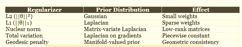
The Bayesian perspective reveals that regularization is not merely a computational trick: it encodes beliefs about the structure of solutions. Choosing L2 asserts that parameters are normally distributed around zero; choosing L1 asserts that most parameters should be exactly zero. These are strong claims that may or may not match the actual structure of the problem.
6. Identifiability and Symmetry
A fundamental question precedes optimization: is the solution unique? If multiple parameter settings produce identical input-output behavior, which one will optimization find, and does it matter?
6.1 Weight Space Symmetries
Neural networks have intrinsic symmetries that create equivalence classes in parameter space:
Permutation symmetry: For any hidden layer with n neurons, there are n! equivalent networks obtained by permuting neurons (and correspondingly permuting incoming and outgoing weights). A network with layers of width [784, 256, 128, 10] has 256! × 128! ≈ 10⁵⁰⁷ equivalent parameterizations.
Scaling symmetry: For ReLU networks, if we multiply incoming weights to a neuron by α > 0 and divide outgoing weights by α, the function is unchanged. This creates a continuous family of equivalent solutions.
Sign symmetry: For networks with tanh activation, flipping signs of incoming and outgoing weights simultaneously preserves the function. This doubles the number of equivalences.
These symmetries have consequences. Gradient descent in the full parameter space wastes capacity exploring equivalent solutions. Loss landscapes appear more complex than they are: many apparent local minima are actually the same solution in different coordinates. Model comparison (asking whether two trained networks learned the same function) requires symmetry-aware distance metrics.
6.2 Quotient Manifold Optimization
The principled solution is to optimize over the quotient space Θ/G, where G is the symmetry group. Points in the quotient represent equivalence classes of parameters, not individual parameter vectors.
Quotient manifold optimization is well-developed in Riemannian geometry. Algorithms exist for computing geodesics, parallel transport, and gradients in quotient spaces. These techniques are standard in computer vision (optimization over rotation groups) and signal processing (optimization over subspace arrangements). Their absence from neural network training is an implementation gap, not a theoretical one.
6.3 Symmetry Breaking for Identifiability
An alternative to quotient optimization is explicit symmetry breaking: adding constraints that select a unique representative from each equivalence class.
Ordering constraints: require that neurons within a layer are ordered by some criterion (e.g., decreasing norm of incoming weights). Eliminates permutation symmetry.
Normalization constraints: require that incoming weight vectors have unit norm. Eliminates scaling symmetry but changes the effective architecture.
Sign conventions: require that the first nonzero element of each weight vector is positive. Eliminates sign symmetry.
These constraints are rarely applied because commercial frameworks don’t surface them as options. The result is that optimization explores a space orders of magnitude larger than necessary, and model comparison requires expensive alignment procedures that could be eliminated by construction.
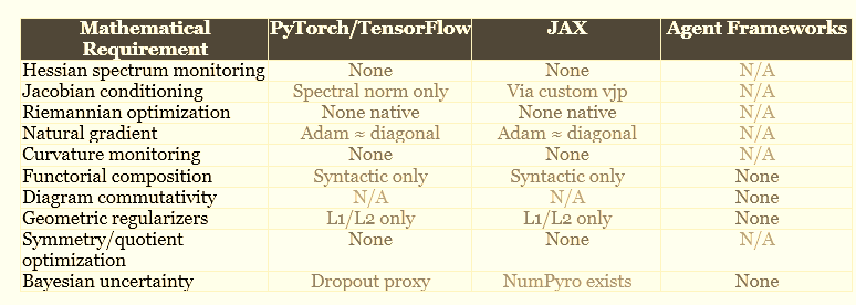
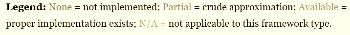
7. The Gap Analysis: Commercial Stacks vs. Mathematical Necessity
We now have the vocabulary to perform a precise gap analysis. The following table maps mathematical requirements to their implementation status in major commercial frameworks.
8. Consequences of the Gaps
These mathematical omissions are not academic concerns. They manifest as concrete failures in production systems.
8.1 Training Instability
Without spectral monitoring, training failure is detected only after it happens—when loss diverges or gradients explode. The warning signs (deteriorating condition numbers, clustering eigenvalues, growing spectral radius) are invisible. Practitioners resort to learning rate schedules and gradient clipping as blind interventions, tuning hyperparameters without understanding what they control.
A spectrally-aware training loop would compute lightweight spectral estimates at checkpoints and adjust optimization strategy proactively. If the Hessian’s condition number exceeds a threshold, switch to preconditioned methods. If Jacobian singular values drift from unity, apply spectral normalization.
These are well-understood techniques applied reactively after trial and error; they should be applied automatically based on measured quantities.
8.2 Unexplained Generalization Failures
Models that achieve low training loss sometimes fail catastrophically on held-out data. Without geometric analysis, this failure is mysterious. With geometric analysis, the explanation is often clear: the model found a sharp minimum (large Hessian eigenvalues) that doesn’t generalize, or the learned representation has pathological curvature that amplifies distribution shift.
Sharpness-aware minimization (SAM) addresses this partially by explicitly seeking flat minima. But SAM is a heuristic; the principled approach is to constrain optimization to remain in regions of bounded curvature throughout training, not merely to prefer flatness at convergence.
8.3 Adversarial Vulnerability
Adversarial examples exist because neural networks invert small singular values, amplifying imperceptible input perturbations into large output changes. This is the Picard condition in reverse: the network’s effective operator has spectral components that grow rather than decay.
Lipschitz constraints (bounding the spectral norm of each layer) provably limit adversarial vulnerability. But current implementations apply these constraints layer-by-layer without accounting for how layer spectra combine through composition. The end-to-end Lipschitz constant can exceed the product of layer constants due to alignment of principal directions—a phenomenon invisible without compositional spectral analysis.
8.4 Agent Incoherence
Multi-agent systems built on LangChain or similar frameworks exhibit emergent pathologies: circular reasoning, inconsistent tool use, memory corruption, and semantic drift over long interactions. These are not bugs in the traditional sense: they are consequences of composing operations without compositional semantics.
A categorically-grounded agent framework would specify which compositions must commute and verify commutativity or fail explicitly. The current approach is to hope that empirical testing catches inconsistencies: a strategy that fails for the long tail of rare but catastrophic interaction patterns.
9. Why the Gap Persists: Structural Explanations
The mathematics described in this paper is not new. Inverse problems, Riemannian optimization, and category theory have decades of development. Why hasn’t this knowledge transferred to AI practice?
9.1 Scaling Obscures Mathematical Sins
The empirical success of large language models creates a selection effect against mathematical rigor. If brute-force scaling solves problems that principled methods would also solve, and scaling is funded while principled methods are not, the field optimizes for scale.
This is a temporary reprieve. Scaling laws plateau. Hardware improvements slow. Eventually the field will need to extract more capability from fixed compute budgets, and mathematical efficiency will matter. The question is whether the mathematical infrastructure exists when it’s needed.
9.2 Disciplinary Silos
Inverse problems expertise resides in applied mathematics departments, typically in the context of medical imaging, geophysics, or signal processing. Differential geometry expertise resides in pure mathematics or theoretical physics. Category theory expertise resides in logic, programming language theory, or pure algebra. None of these communities have significant overlap with machine learning engineering.
PhD programs in machine learning train students in optimization, statistics, and software engineering. The mathematical prerequisites do not include functional analysis beyond basic Hilbert spaces, Riemannian geometry beyond the definition of a manifold, or category theory at all. The expertise gap is structural.
9.3 Abstraction Debt
Implementing Riemannian optimization requires abstractions that don’t exist in commercial frameworks: manifold objects, tangent space representations, Riemannian metrics, parallel transport operators, geodesic solvers. Building these on top of tensor libraries is possible but requires invasive modifications that break existing workflows.
Category theory is worse: no mainstream programming language has native support for functors, natural transformations, or diagram verification. Implementing categorical structure requires either embedding in a dependently-typed language (impractical for production) or building custom verification tools (expensive and maintenance-intensive).
The abstractions that would make principled methods practical require infrastructure investment that no individual company has incentive to provide. This is a coordination problem: everyone would benefit from the infrastructure, but no one wants to build it.
9.4 Incentive Misalignment
Academic incentives reward novelty over foundations. Papers that introduce new spectral monitoring methods for existing architectures are less publishable than papers that introduce new architectures. The mathematical scaffolding is “not novel enough” for top venues, so researchers avoid building it.
Industry incentives reward shipping over correctness. A product that works 90% of the time is shippable; a principled system that works 95% of the time but takes twice as long to build is not. The 5% improvement doesn’t justify the investment, even though the failure modes in the remaining 10% vs 5% may be qualitatively different.
10. Toward a Mathematically Complete AI Stack
What would a mathematically principled AI framework look like? This section sketches the requirements without claiming implementation details.
10.1 Spectral Dashboard
Every training run should expose real-time estimates of: Hessian condition number and spectral density, layer-wise Jacobian singular value distributions, end-to-end Lipschitz constant estimates, and Picard condition violations (where data has components in spectral directions the model cannot represent).
These quantities should trigger automatic interventions: preconditioner updates when conditioning deteriorates, spectral normalization when singular values drift, architecture modifications when Picard violations persist.
10.2 Geometric Optimization Engine
The optimizer should understand parameter manifolds natively. Weight matrices with orthogonality constraints should be updated via Riemannian gradient descent on the Stiefel manifold. Probability distributions should be updated via natural gradient with Fisher-Rao metric. Quotient structures from symmetries should be handled automatically.
The API should accept manifold specifications declaratively: “these parameters lie on SO(n)” or “these parameters are equivalent up to permutation.” The optimizer should compute appropriate geodesics, retractions, and parallel transport without user intervention.
10.3 Regularization Library
Beyond L1/L2, the framework should provide: total variation and higher-order Sobolev penalties, nuclear norm and general Schatten p-norms, geodesic regularization for manifold-valued parameters, curvature bounds on learned representations, spectral constraints (condition number bounds, spectral gap requirements), and structured sparsity patterns from group theory (block-sparse, hierarchical-sparse).
Each regularizer should have an associated Bayesian interpretation exposed to the user, making explicit the prior assumptions encoded by the choice.
10.4 Compositional Agent Framework
Agent orchestration should be specified as diagrams with explicit commutativity requirements. The framework should verify at construction time that specified diagrams commute (for deterministic operations) or fail with informative errors explaining which paths diverge.
Stateful operations should be explicitly marked and tracked through composition. Memory updates should preserve declared invariants. Tool calls should satisfy contracts specified in typed interfaces with semantic content, not just syntactic shape.
11. Conclusion
Commercial AI frameworks implement a fragment of the mathematics that governs learning systems. The omissions are not random; they cluster around the mathematical domains that address instability, ill-posedness, and compositional semantics: precisely the domains needed to make AI systems reliable.
This article has catalogued the gaps: spectral theory for stability and generalization, differential geometry for optimization on curved spaces, category theory for compositional semantics, group theory for identifiability, and regularization theory for well-posedness. Each gap corresponds to a class of unexplained failures in current systems.
The gaps persist due to structural factors: scaling success that obscures mathematical necessity, disciplinary silos that prevent knowledge transfer, abstraction debt that makes principled methods impractical, and incentives that reward shipping over correctness.
Closing these gaps requires coordinated investment in mathematical infrastructur: the kind of investment that benefits everyone but no one wants to fund. The alternative is to continue building on incomplete foundations, accepting that certain classes of failures are endemic rather than solvable.
For practitioners: the immediate implication is that unexplained training failures, generalization anomalies, and agent incoherence are often symptoms of mathematical pathologies that existing tools cannot diagnose. The path forward is to develop fluency in the missing mathematics and apply it to understand (if not yet fix) the systems we build.
For the field: the call is to recognize that inverse problems are the natural mathematical framing for machine learning, and to import the century of theory developed for inverse problems into AI practice. The mathematics exists. The engineering challenge is to make it practical.
References
Hadamard, J. (1923). Lectures on Cauchy’s Problem in Linear Partial Differential Equations. Yale University Press.
Tikhonov, A. N., & Arsenin, V. Y. (1977). Solutions of Ill-Posed Problems. Winston & Sons.
Amari, S. (1998). Natural gradient works efficiently in learning. Neural Computation, 10(2), 251-276.
Engl, H. W., Hanke, M., & Neubauer, A. (2000). Regularization of Inverse Problems. Springer.
Absil, P. A., Mahony, R., & Sepulchre, R. (2008). Optimization Algorithms on Matrix Manifolds. Princeton University Press.
Stuart, A. M. (2010). Inverse problems: A Bayesian perspective. Acta Numerica, 19, 451-559.
Sagun, L., Bottou, L., & LeCun, Y. (2016). Eigenvalues of the Hessian in deep learning: Singularity and beyond. arXiv:1611.07476.
Dinh, L., Pascanu, R., Bengio, S., & Bengio, Y. (2017). Sharp minima can generalize for deep nets. ICML.
Ghorbani, B., Krishnan, S., & Xiao, Y. (2019). An investigation into neural net optimization via Hessian eigenvalue density. ICML.
Yao, Z., Gholami, A., Keutzer, K., & Mahoney, M. W. (2020). PyHessian: Neural networks through the lens of the Hessian. IEEE Big Data.
Bronstein, M. M., Bruna, J., Cohen, T., & Veličković, P. (2021). Geometric Deep Learning: Grids, Groups, Graphs, Geodesics, and Gauges. arXiv:2104.13478.
Cohen, J., Kaur, S., Li, Y., Kolter, J. Z., & Talwalkar, A. (2021). Gradient descent on neural networks typically occurs at the edge of stability. ICLR.