

THE TWO ALGEBRAS FOR AI - AND WHY EVERYONE USES THE WRONG ONE
Build Worlds, Not Limits: The Jet Algebra Playbook.

TL;DR — ADVANCED MATH IN AI FOR DUMMIES 😃
The claim: 19th-century, limit-based calculus is the wrong algebra for machines. It fakes infinitesimals and forces step-size roulette.
The fix: Use true infinitesimals in spirit (hyperreals) and their CPU-ready engine (dual/jets). Derivatives and curvature become structural, not a side-procedure.
What this post give you (fast):
A one-screen recipe to replace finite differences with dual numbers (value + JVP in one pass).
A 2-lane upgrade with jets (k=2) for cheap HVP/Newton/TR—curvature on tap, no full Hessian.
A practical checklist to debug any model via per-layer
(value, JVP, …)and to prune/quantize by curvature, not vibes.
What you get (outcomes, not vibes):
Fewer, stabler steps (2–5× on hard losses).
Less wobble (no step-size guessing, no FD noise).
Smaller, sharper models (50–90% prunes with tiny loss hits, task-dependent).
Cleaner reasoning when paired with geometric memory/routing (toroid keys) and hierarchical reps (hyperbolic).
The deal:
Give me five minutes. I’ll replace epsilon-delta theater with an algebra your GPU actually understands: carry the derivatives, see the shape, train faster.
The limit-based calculus currently used in AI operates entirely in
and thus fake infinitesimals.
Cauchy and Weierstrass screwed up how we analyze continuous functions by replacing infinitesimals with limits:
The now–popular derivative comes from that swap: fake infinitesimals implemented via limits:
In their time, it was an advance—no doubt. Replacing Newton’s fluents/fluxions and Leibniz’s infinitesimals with limit-based calculus was an acceptable workaround. But in the 21st century—where we automate calculus over billions of parameters—the limit-based approach is atrociously obsolete, and it’s the real bottleneck to building decent AI.
The irony? We’re circling back to the original insight shared by both founders: calculus should be grounded in numbers that capture the “infinitely small.” Newton framed it dynamically (fluents/fluxions as flowing quantities and their instantaneous rates). Leibniz worked algebraically with infinitesimals. Three centuries later, hyperreals give those infinitesimals a rigorous foundation, and on machines we should use their finite engines—dual and jet algebras - to carry derivatives (and curvature) directly through computation.
THE SHOWDOWN: TRUE INFINITESIMALS vs FAKE LIMITS
How true infinitesimals fix the failures
Now we step onto the solid ground of number theory and algebra, leaving behind the 19th-century, limit-based mirage that has ruled calculus — and, tragically, still rules modern AI, with all the catastrophic consequences we see in its four error types.
Forget the flat number line of the Real Numbers.
That line was the foundation of the old Archimedean empire — a world where everything had to be measured by stacking finite steps, and where “limits” were invented to fake what infinitesimals actually are.
But we no longer have to pretend.
We’re entering a new mathematical universe — the Hyperreal Numbers Universe — the long-overdue replacement for the Real Number system on which today’s AI algebra is fatally built.
The Real Numbers can’t represent infinitesimals or true infinities. They flatten everything into one fragile, linear scale. And that’s exactly why AI keeps breaking — oscillating between vanishing gradients and exploding values, the four classic error types of a geometry that can’t see beyond its own horizon.
The Hyperreal field fixes this.
It restores the full spectrum of scale — from the infinitesimally small to the infinitely large — and gives calculus back its missing architecture.
Stop for a moment and picture that.
A number system wide enough to handle every scale that nature — and intelligence — can throw at it.
In its simplest, metaphorical form, this new mathematical universe appears as a row of galaxies, each a distinct realm of magnitude.
Now you’re ready to explore Chart 1 below — a visual introduction to the Hyperreal Numbers Universe, shown here in its most intuitive, creative form: a row of galaxies.
Each disk represents an entire realm of numbers contained in the Hyperreal superset — the extended number system that includes all reals, plus the infinitesimal and infinite magnitudes the reals could never hold.
Each disk represents an entire realm of numbers contained in the Hyperreal superset:
Galaxy ε on the left — the infinitesimal cloud, where numbers are smaller than any real yet still not zero.
Galaxy ℝ in the middle — home to all ordinary reals and their infinitesimal halos (the Monads of 1, π, e …).
Galaxy ω on the far right — the infinite realm that no finite number can ever reach.
The dashed axis isn’t a ruler; it’s a logical thread ordering the galaxies from the infinitely small to the infinitely large. Distances here mean nothing. Only hierarchy survives.

But that row of galaxies was only a teaser.
It shows where each realm sits, but not how they connect. The Hyperreal Universe isn’t flat — it’s layered. Think less “line,” more onion of scales, each world wrapped inside another.
Here’s the main idea to understand the charts: those distances mean nothing.
You can’t slide from ε to 1, or from 1 to ω, by taking steps. The Archimedean ruler — the idea that everything can be reached by adding enough finite pieces — breaks here. Geometry collapses; only order remains.
That’s what Chart 2 reveals.
If Chart 1 showed the map, Chart 2 reveals the laws of hyperreal gravity — how the entire Hyperreal Universe holds together around its silent core, 0.
The galaxies stop lining up and start nesting. The infinitesimal cloud (Galaxy ε) sits at the center, surrounded by the finite realm (Galaxy ℝ), which itself is engulfed by the infinite galaxies (ω, ω², …).
Chart 2. The Nested, Pulsating Galaxies of the Hyperreal Numbers Universe. An animated view of the hierarchy of scale inside the hyperreal field. Every orbit revolves around 0, the symbolic core of all monads. Galaxy ε forms the infinitesimal cloud, Galaxy ℝ the finite realm of limited magnitudes (all real numbers and their halos), and Galaxy ω the domain of infinite values beyond reach. The pulsating halos mark the living frontiers between realms—approached through endless refinement but never crossed by finite steps. They replace static Archimedean distance with motion in time, turning geometry into the rhythm of the infinite.
Hyperreals in Action For Programmers
We’ve now seen the shape of the hyperreal universe.
But to turn that geometry into usable algebra: something programmable, differentiable, and verifiable. We must formalize what lives inside each “galaxy” of numbers.
1. The Definition That Newton Dreamed Of
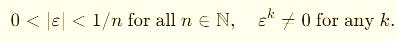
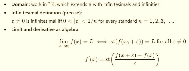
Work inside ∗R: the real numbers extended with non-zero infinitesimals.
Here’s the compact definition that took mathematics three centuries to rediscover:
No limits. No guessing. Just a number smaller than any fraction of reals: a true infinitesimal.
This single idea resurrects Newton’s intuition and fixes the broken calculus that modern AI still runs on.
2. The Taxonomy of Fields Inside the Hyperreal Superset
(Or: the four number systems every serious AI engineer should secretly be using)
Let’s get practical.
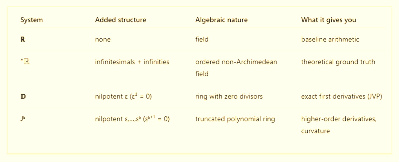
Behind all that galaxy talk, we’re really dealing with four kinds of numbers — the ones that can actually change the way we build and train AI.
Each of these number systems — real, hyperreal, dual, jet — forms its own algebraic habitat, obeying different group, ring, and field laws.
They’re not abstract nonsense; they’re layers of algebra that shape how your program handles motion, precision, and learning.
Think of them as four habitats in one mathematical ecosystem, each with its own physics — from the plain reals we’ve always used, to the hyperreals that define infinitesimals, down to the duals and jets that finally make all this computable.
One Universe, Four Number Forces
At the center sits the real numbers (ℝ) — the baseline arithmetic of every model and matrix multiply.
Extend them once, and you get the hyperreals (∗R^*\mathbb{R}∗R), the true mathematical universe that contains both infinitesimals and infinities.
Project a simplified, finite version of that same idea, and you arrive at the dual numbers (𝔻) and jets (Jᵏ) — the algebraic workhorses that make automatic differentiation possible.
In the set-theoretic view (see the Venn diagram),
ℝ embeds naturally inside each extension:
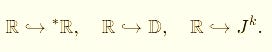
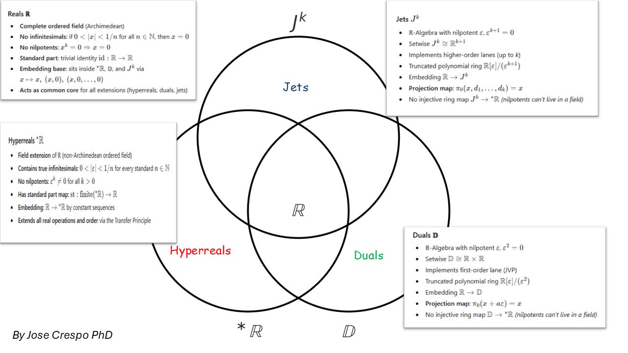
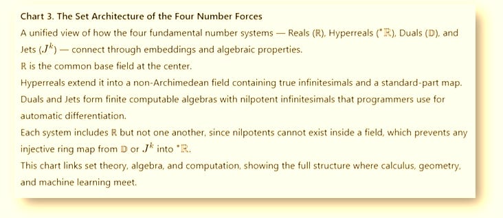
All four live in the same universe of structure — but their rules differ radically.
To Be or Not to Be Nilpotent
Here’s where the roads split.
Hyperreals (∗R)
A field, perfectly ordered, no zero divisors.
That means no nilpotents — no “magic” numbers that vanish when squared or cubed.
Their infinitesimals ε are real elements in the algebraic sense:
They’re tiny — smaller than any real fraction — but never zero.
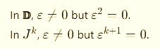
Duals (𝔻) and Jets (Jᵏ)
These are rings, not fields, and they do contain nilpotents — elements that die after a few powers.
These nilpotents are algebraic doppelgängers of infinitesimals: not “real” in a field-theoretic sense, but powerful tools for derivatives.
They gauge infinitesimal behavior just enough to automate calculus inside your code.
So the fact that nilpotents exist in duals/jets but are forbidden in the hyperreals is the deep structural divide.
Hyperreals: true infinitesimals, no nilpotents.
Duals & Jets: nilpotent “gauged infinitesimals,” no field structure.
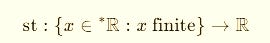
Standard Part vs. Projection — How They “Return” to Reals
Now, how do we come back to normal reals after playing in these extended worlds?
In the hyperreals, we use the standard-part map:

It collapses the infinitesimal halo:
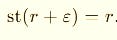
That’s the real number your hyperreal was infinitely close to.
In duals and jets, there’s no notion of “infinitely close,” because these are algebraic rings, not ordered fields.
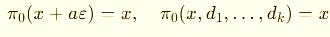
So we use the simpler projection:
In plain English: just grab the value lane and ignore the derivative lanes.

Programmer shortcut:
st(·) → “take the real shadow” (hyperreals).
π₀(·) → “take the first component” (duals/jets).
In ∗R, infinitesimals are real field elements, with true proximity and a genuine standard part.
In 𝔻 and Jᵏ ε-parts are nilpotent coefficients that vanish by projection — no infinite closeness, just algebraic bookkeeping.
Why This Matters for AI
Hyperreals give us the ideal semantics of calculus — the way derivatives and limits were meant to behave before we replaced them with fragile ε–δ tricks.
Duals and jets give us the machine algebra to compute those derivatives exactly, without symbolic headaches or numerical jitter.
When you lift a real input x into a jet:
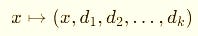
and run your usual forward pass,
you’re literally running your program over a truncated Taylor ring.
At the end, you project back — value in lane 0, gradient in lane 1, curvature in lane 2, and so on.
That’s how real code gets exact calculus.
So here’s the simple rule of thumb:
Hyperreals explain calculus.
Duals and jets compute it.
The first gives meaning, the second gives power.
ALGEBRA: THE RULES TO PLAY THE AI GAME WITH HYPERREALS
Alright, time to stop orbiting theory and touch the ground.
We’ve mapped the four Number Forces — Reals, Hyperreals, Duals, and Jets.
Now we build the algebra that actually makes them move.
This is where abstract structure turns into computation.
The Hyperreals give you the truth of calculus — infinitesimals included.
Duals and Jets give you the machinery — the algebraic engines that make that truth computable.
Think of it like this:
Hyperreals are the blueprint.
Duals and Jets are the compiler.
We’ll move step by step: from pure infinitesimals to first derivatives to curvature.
By the end, you’ll see that automatic differentiation — the core of modern AI — is nothing more than hyperreal algebra disguised as code.
1. Hyperreal Infinitesimals — the Conceptual Ground Truth
Here, st(·) means standard part: it removes the infinitesimal tail.
We don’t simulate ∗R directly: we build a finite algebra that reproduces its derivative behavior exactly.
2. Dual Numbers (K = 1)
Elements:
x̂ = x + d1*ε with ε² = 0Arithmetic:
(x + a*ε) + (y + b*ε) = (x + y) + (a + b)*ε
(x + a*ε) * (y + b*ε) = (x*y) + (x*b + a*y)*ε     # product rule appears
Constants lift as (c, 0).
Functions (first order)
The coefficient of ε is the directional derivative (JVP):
For smooth f:
f(x + d1*ε) = f(x) + f’(x)*d1*ε
Programming recipe
Represent a scalar as
(x, d1).Set
d1 = 1to get ∂f/∂x, or use a direction vectorvto getJf(x)·v.Implement
+and*once — everything else flows automatically.
Cost: about 2–3× a normal forward pass.
3. Jets (K = n ≥ 2)
Duals give you slopes. Jets give you curvature and higher-order awareness.
Elements:
x̂ = x + d1*ε + (d2/2!)*ε² + ... + (dn/n!)*εⁿ
with εⁿ⁺¹ = 0
Arithmetic (up to order 2):
(Ax, A1, A2) * (Bx, B1, B2) =
( Ax*Bx,
  A1*Bx + Ax*B1,
  A2*Bx + 2*A1*B1 + Ax*B2 )
Functions (order n):
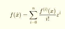
Each power of ε carries one derivative order.
It’s like a multi-lane Taylor engine where curvature, acceleration, and higher changes flow in parallel.
Why this matters
Jet² gives Hessian-vector products (HVPs) and Newton/TR steps without explicitly building a Hessian.
Higher-order Jets (J³, J⁴, …) give full Taylor expansions in one pass — vital for control, simulation, and meta-learning.
From 19th-Century Limits based calculuus to 21st-Century Hyperreal Algebra
Okay, take a breath.
This is where algebra finally turns into code.
If you’ve ever watched PyTorch or JAX mysteriously “find gradients,” you’ve already seen this in action: We can go beyond that - with far fewer lines of code - using hyperreal algebra running quietly behind the curtain.
Duals and Jets will give your program extra “lanes” of motion:
one for value, one for slope, and more for curvature.
What looks like magic is simply the algebra of ε doing its job.
Let’s meet the three fundamental operators that make all of AI calculus work:
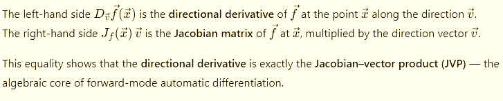
1.- JVP — Forward Mode
Imagine you nudge your input x slightly in a direction vector
The Jacobian–vector product (JVP) tells you how the function f(x) immediately responds:
That’s just the first derivative of f in the direction of v.
In derivative notation we have:
In practice, dual numbers do this automatically:
seed  x̂ = x + v·ε
run   f(x̂)
read  coefficient of ε  →  Jf(x)·v
That’s forward-mode autodiff in a nutshell — fast when inputs are small, exact by design.
What does that actually mean?
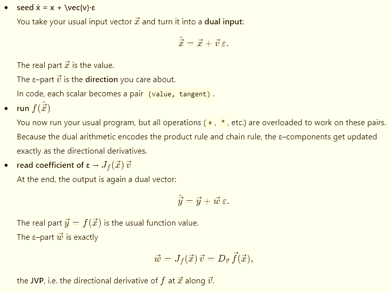
So forward-mode autodiff is nothing mysterious:
Wrap your inputs as duals, run the same code, and read the ε–lane.
The ε–lane is the first derivative in the chosen direction.
It’s fast when the input dimension is small, and exact up to floating-point because every step is just algebra, not numerical approximation.
2.- VJP — Reverse Mode
Now flip the flow.
You already know the final result (say, a scalar loss).
You want to know how each input contributed to it.
We have to use for that the vector–Jacobian product (VJP):

Here ∇f (the nabla) is the gradient of the output with respect to the network’s final value — the direction of steepest ascent. Backprop/VJP computes this gradient. The optimizer then flips the sign and uses −∇f to follow the steepest descent path on the loss.
VJP propagates this gradient backward, layer by layer, revealing how each parameter influences the result.
That’s the real math behind backprop.
NOTE:
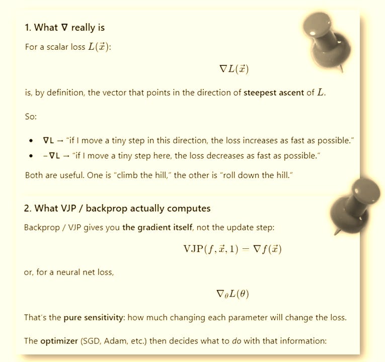
The optimizer (SGD, Adam, etc.) then decides what to do with that information:
θ_new = θ_old - η * ∇θ L(θ_old)The minus sign lives in the update rule, not inside the gradient itself.
So:
VJP/backprop → computes ∇L (steepest ascent).
Gradient descent → uses −∇L to actually step downhill.
3.- Now for the Third Basic Operator — The Hessian–Vector Product (HVP)
We finally bring out the heavy artillery: group theory and composition laws.
Before coding curvature, we need to understand its algebra—because curvature is just the second composition of derivatives. In familiar language, this means: the second derivative, but computed the way AI actually does it—with category theory and jet algebra, not 19th-century limits.
Why Group Theory Comes First
Every neural network is just a gigantic chain of functions:
Group theory (and its cousin 😁 , category theory) tells us something profound:
If you can define how a single layer transforms its inputs and derivatives,
the composition of those layers automatically defines the behavior of the entire network.
So in plain english:
once you specify how a single layer transforms values and their ε*-lane (derivatives), the entire network’s derivative behavior follows by composition.
This is why, if you are a developer or engineer working on AI, it’s now a big blunder not to know anything about Category Theory (composition). You can simplify your code in extensibility and efficiency, doing things otherwise impossible.
For example, the very useful second derivative for AI is a very tough task, further penalized by a huge performance cost (hence why current LLMs rarely use it, despite its potential to greatly reduce hallucinations).
Yet it becomes a trivial operation and an easy performance win if you, as a programmer with some idea of Category Theory, use a simple composition of two first-derivative (k=1 duals) operators—JVP and VJP—to get it “for free,” without using the more expensive (k=2) jet.
How Self-driving Tesla Car could fix most of their mistakes:
Apparently not even Tesla seems to not anything about using this maths to solve most of its self-driving cars.
.This is why you sometimes see Tesla videos where the car:
Brakes suddenly for no apparent reason
Takes curves too fast and has to correct
Makes jerky steering adjustments
Does things that make passengers go “Why did it just do that?”
The car is reacting to what’s happening right now, not anticipating what’s about to happen.
Tesla could easily solve these problems by using second derivatives: Hessian-vector products (HVP). But Tesla engineers, like everyone else, still use 19th-century limit-based calculus instead of dual/jet numbers that make HVP a computationally trivial operation, using the composition of two first-order operators (JVP ∘ VJP) to get HVP directly.
The killer insight: You can compose two first-order operators (JVP and VJP) to get second-order information (HVP)—but only if derivatives are algebraic objects (hyperreals), not numerical approximations (h-limit calculus).
See it in code. With dual/jet numbers you operate with algebra—easy peasy to get the right functor through composition of two first derivatives:
See that in the code:
With dual/jet numbers (algebraic):Clean, composable, exact. This is why modern AI can be efficient.
hvp = vjp(lambda x: jvp(f, (x,), (v,))[1], x)[1](u)[0] # Exact
With finite differences (19th-century approach):
# Must nest approximations—structurally non-functorial
hvp_fd = ((f(x+h_prime*u+h*v) - f(x+h_prime*u))/h
          - (f(x+h*v) - f(x))/h) / h_prime  # Coupled errors
What’s wrong with this code?
Let me translate what this mess actually does:
You have to guess two magic numbers (
handh_prime) - and there’s no right answerYou’re computing approximations of approximations - errors multiply
You can’t combine simple operations - no composition, no reuse
It’s slow - you have to evaluate the function 4+ times just to get one answer
It’s fragile - tiny changes in
hgive wildly different results
The Real-World Translation
Imagine you’re trying to figure out if the road ahead curves by:
Driving forward a little bit (
h) and checkingThen driving sideways a little bit (
h_prime) and checking againThen doing some complicated subtraction to guess the curve
Meanwhile, the road is right there. You could just look at it properly!
That’s what the old math does - it takes something that should be straightforward and turns it into a guessing game with multiple moving parts that can all go wrong.
Why This Causes Self-Driving Disasters
This tangled, fragile code is why you see:
❌ Phantom braking (the errors made it think there’s a curve)
❌ Jerky steering (constantly correcting because the approximation was wrong)
❌ Dangerous situations (by the time it figures out the real curve, it’s too late)
The problem isn’t that engineers are bad—it’s that they’re using 19th-century tools for 21st-century problems.
BEYOND the CURVES at K=2 at welcome to the real physical world realistic simulation with K= 3
So using the example of Self-driving cars you have got the substance idea why you have to get rid of the old calculus and embrace the new algebra based calculus.
Is the algebra based calculus (realistic feasible by using dual/jet numbers) that makes very cheap using the Second-Order thinking or solving most of the problems of all machines powered by AI.
Explained without math:
Step 1: Add “Curve Detection” (The HVP Magic)
Instead of just asking “Which way?”, the car should also ask:
“How sharply is this direction about to change?”
Real-world analogy:
First-order (current Tesla): “The road is tilting left” → Turn left
Second-order (what we need): “The road is tilting left, and that tilt is getting steeper fast” → Turn left and slow down
This “how fast is the direction changing” is called curvature, and it’s what you get from a second derivative.
The Clever Trick: Two Simple Checks = One Complex Answer
Here’s again in plain english where the composition magic comes in (explained without the math):
Old way 19 century formula (impossible): Try to compute how the entire road curves everywhere all at once
Like trying to draw a complete map of every turn ahead
For a Tesla-sized AI: Would require more memory than exists on Earth
New way (the composition trick): Combine two simple questions:
“If I move forward a tiny bit, where do I end up?” (JVP)
“If I ended up there, which direction would I need to go?” (VJP)
When you chain these two simple questions together, you automatically get the answer to: “How sharply am I about to turn?”
Key insight: Each question alone is cheap and simple. But their combination tells you something complex—curve sharpness—without having to compute it directly.
Why This Prevents Mistakes
Scenario 1: The Phantom Brake
Current Tesla:
Sees shadow on road
Shadow makes road look different
Thinks “road is changing → brake!”
Passenger: “Why did we just brake for nothing?”
With second-order (HVP):
Sees shadow on road
Checks: “Is the road curving or just shaded?”
Shadow doesn’t change curvature (road is still straight)
Car: “False alarm, keep going”
Passenger: Smooth ride, no sudden braking
Scenario 2: The Sharp Turn
Current Tesla:
Approaching curve at 45 mph
System: “Road is straight... still straight... still straight... OH CRAP IT’S TURNING!” 💥
Sudden brake + hard steer
Passenger gets jerked around
With second-order (HVP):
Approaching curve at 45 mph
System: “Road is straight, but the rate of change is increasing”
Translation: “A curve is coming”
Gradual deceleration before the turn
Smooth steering through the curve
Passenger: Comfortable ride
Step 2: The “Sanity Check” (Third-Order Verification). Welcome to the K=3 world
But we can go one step further. Add a tiny verification system that asks:
“Does everything make sense together?”
What it checks:
Lane lines: Do they curve the same way as the road curvature predicts?
Road signs: Does the “sharp curve ahead” sign match what we’re detecting?
Other objects: Are pedestrians/cars behaving like the road goes where we think it goes?
If the story doesn’t add up → VETO the action
Example:
Car detects sharp right turn coming
But lane lines show slight left curve
Street sign says “Curve Left Ahead”
Mismatch detected!
System: “Something’s wrong with my curve calculation, better slow down and be careful”
This is the k=3 (third-order) verification—it checks if all the different measurements are consistent with each other. And only JET Numbers can do that miracle. More in the next article.
Driving forward a little bit (
h) and checkingThen driving sideways a little bit (
h_prime) and checking againThen doing some complicated subtraction to guess the curve
Meanwhile, the road is right there. You could just look at it properly!
That’s what the old math does - it takes something that should be straightforward and turns it into a guessing game with multiple moving parts that can all go wrong.
Why This Causes Self-Driving Disasters
This tangled, fragile code is why you see:
❌ Phantom braking (the errors made it think there’s a curve)
❌ Jerky steering (constantly correcting because the approximation was wrong)
❌ Dangerous situations (by the time it figures out the real curve, it’s too late)
The problem isn’t that engineers are bad—it’s that they’re using 19th-century tools for 21st-century problems.
BEYOND CURVES (k=2): Welcome to the Real Physical World with k=3
Okay, so we’ve talked about detecting curves (that’s the k=2 world - second derivatives). But the real world is messier than just curves.
Here’s the big idea:
Using the self-driving car example, you now understand why you need to abandon old calculus and embrace the new algebra-based calculus.
It’s this algebra-based calculus (made realistic by using dual/jet numbers) that makes “Second-Order Thinking” cheap and practical—solving most problems in all machines powered by AI.
Let me break this down into plain English, keeping all our dance steps to the rhythm of the AI music.
Step 1: Add “Curve Detection” (The HVP Magic)
Instead of just asking “Which way should I go?”, the car should also ask:
“How sharply is this direction about to change?”
Real-World Analogy
First-order thinking (current Tesla):
“The road is tilting left” → Turn left
Like looking at your feet while walking
Second-order thinking (what we need):
“The road is tilting left, and that tilt is getting steeper fast” → Turn left and slow down
Like looking 20 feet ahead while walking
This “how fast is the direction changing” is called curvature, and it’s what you get from a second derivative.
The Clever Trick: Two Simple Checks = One Complex Answer
Here’s where the composition magic comes in (no math this time, I promise):
Old way (19th-century formula) - IMPOSSIBLE:
Try to compute how the entire road curves everywhere all at once
Like trying to draw a complete map of every turn ahead while driving
For a Tesla-sized AI: Would require more memory than exists on Earth
This is why nobody does it this way anymore
New way (the composition trick) - PRACTICAL:
Combine two simple questions:
“If I move forward a tiny bit, where do I end up?” (JVP)
“If I ended up there, which direction would I need to go?” (VJP)
When you chain these two simple questions together, you automatically get the answer to:
“How sharply am I about to turn?” And boom that’s your Hessian–Vector Product (HVP).
Key Insight
Each question alone is cheap and simple. But their combination tells you something complex—curve sharpness—without having to compute it directly.
It’s like:
Instead of trying to predict tomorrow’s weather by simulating every air molecule
You just check: “What’s the temperature now?” + “How fast is it changing?”
Boom - you know if a storm is coming
Why This Prevents Real Mistakes
Scenario 1: The Phantom Brake Problem
Current Tesla (first-order only):
Sees shadow on road
Shadow makes the road look different
System thinks: “Road appearance changed → Something happened → BRAKE!”
Passenger: “Why did we just brake for nothing?!”
With second-order (HVP added):
Sees shadow on road
Checks: “Is the road curving or just shaded?”
Shadow doesn’t change the curvature (road is still straight)
System: “False alarm—it’s just a shadow. Keep going.”
Passenger: Smooth ride, no sudden braking
Scenario 2: The Sharp Turn Problem
Current Tesla (reacting, not anticipating):
Approaching curve at 45 mph
System: “Road is straight... still straight... still straight...”
System: “OH CRAP IT’S TURNING!” 💥
Sudden brake + hard steer
Passenger gets jerked around
With second-order (HVP - anticipating):
Approaching curve at 45 mph
System: “Road is straight, but the rate of change is increasing”
Translation in computer brain: “A curve is coming in about 3 seconds”
Gradual deceleration starts before the turn
Smooth steering through the curve
Passenger: Comfortable ride, didn’t even notice
The difference: Reacting vs. Anticipating. That’s what second derivatives give you.
Step 2: The “Sanity Check” (Third-Order Verification)
Welcome to the k=3 Physical World
But we can go even one step further. This is where things get really powerful.
Add a tiny verification system that constantly asks:
“Does everything make sense together?”
This is like having a co-pilot who’s constantly double-checking your work.
What It Checks
Lane lines:
Do they curve the same way the road curvature predicts?
If the car thinks “sharp right turn” but the lane lines show “gentle left curve”
Something is wrong
Road signs:
Does the “Sharp Curve Ahead” sign match what we’re detecting?
If sign says left curve but car detects right curve
Something is wrong
Other objects:
Are pedestrians/cars behaving like the road goes where we think?
If cars ahead are going straight but we think there’s a turn
Something is wrong
The Power Move: Veto Authority
If the story doesn’t add up → VETO the action
The car doesn’t just blindly follow its calculations. It checks if reality agrees.
Real Example
Dangerous situation prevented:
Car’s curve detector: “Sharp right turn coming”
Lane lines: “Actually showing a slight left curve”
Street sign: “Curve Left Ahead”
MISMATCH DETECTED!
System decision: “I don’t trust my curve calculation. Something’s wrong with my sensors or my math.”
Action: Slow down, stay in lane, be extra careful
Result: Avoided a potentially dangerous wrong turn
This is k=3 (third-order) verification - it checks if all the different measurements are consistent with each other.
Think of it like this:
k=1: “Which way is the road going?” (direction)
k=2: “How sharply is it about to curve?” (curvature)
k=3: “Do all my measurements agree about what’s happening?” (consistency check)
Why Only Jet Numbers Can Do This
Here’s the technical truth in simple terms:
Old math (finite differences):
Can barely handle k=1 (direction)
Struggles with k=2 (curves)
Completely breaks down at k=3 (consistency checking)
Like trying to build a skyscraper with duct tape
New math (jet numbers):
Handles k=1 easily (direction)
Handles k=2 efficiently (curves)
Can scale to k=3, k=4, and beyond (full verification)
Like building with proper structural engineering
The Memory Comparison
For a Tesla-sized AI brain:
Old approach at k=3:
Would need more memory than all the computers on Earth combined
Literally impossible
New approach at k=3:
Needs about 3× the memory of basic operation
Totally doable with current hardware
The Performance Comparison
Old approach:
Takes many minutes to compute one decision
Errors everywhere
Unreliable
New approach:
Takes milliseconds
Exact calculations (within computer precision)
Reliable
The Bottom Line for Programmers
If you’re building AI systems (any AI systems), here’s what you need to know:
First-order (k=1): Basic direction - “where should I go?”
This is what most systems do today
It’s not enough
Second-order (k=2): Anticipation - “what’s about to happen?”
This prevents most stupid mistakes
Made practical by composition trick (JVP∘VJP)
Third-order (k=3): Verification - “does everything add up?”
This catches the mistakes that slip through
Only possible with jet numbers, not old math
The choice:
Keep using 19th-century math → keep getting 19th-century results (failures, disasters, “why did it do that?”)
Switch to algebra-based calculus → join the 21st century (reliable, anticipatory, trustworthy AI)
And the beautiful part: The algebra-based approach is actually easier to code once you understand it. The old way looks simpler but is actually a nightmare of guesswork and fragile approximations.
Coming Up Next
The miracle of jet numbers isn’t just that they work—it’s that they make impossible things possible.
See you!
This article comes at the perfect time because your description of 'epsilon-delta theater' as what needs to be replaced with an algebra a GPU naturally understands for faster training is such an incredibly insightful and wonderfully curious consept that makes me think about how we teach math to future AI developers.