Three numbers. That’s all your AI needs to work.

The mathematical diagnostics that have existed since 1950 — and still aren’t in any AI framework

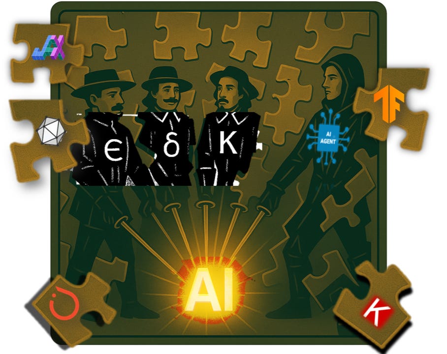
If You Don’t Understand Eigenvalues, You Don’t Understand AI

What if I told you that three numbers — just three — could predict whether your AI will work or catastrophically fail?

No new architecture. No retraining. No infrastructure overhaul.

Just simple math. Math that’s been sitting in textbooks since 1950, waiting for someone to bother checking it.

These three numbers would have caught:

Your Tesla phantom braking for no reason.

GPT-4 citing a court case that doesn’t exist: submitted by a lawyer, who got sanctioned.

Your model, trained for three weeks, beautiful loss curve, shipped to prod, immediately falling on its face.

Same root cause. Every single time.

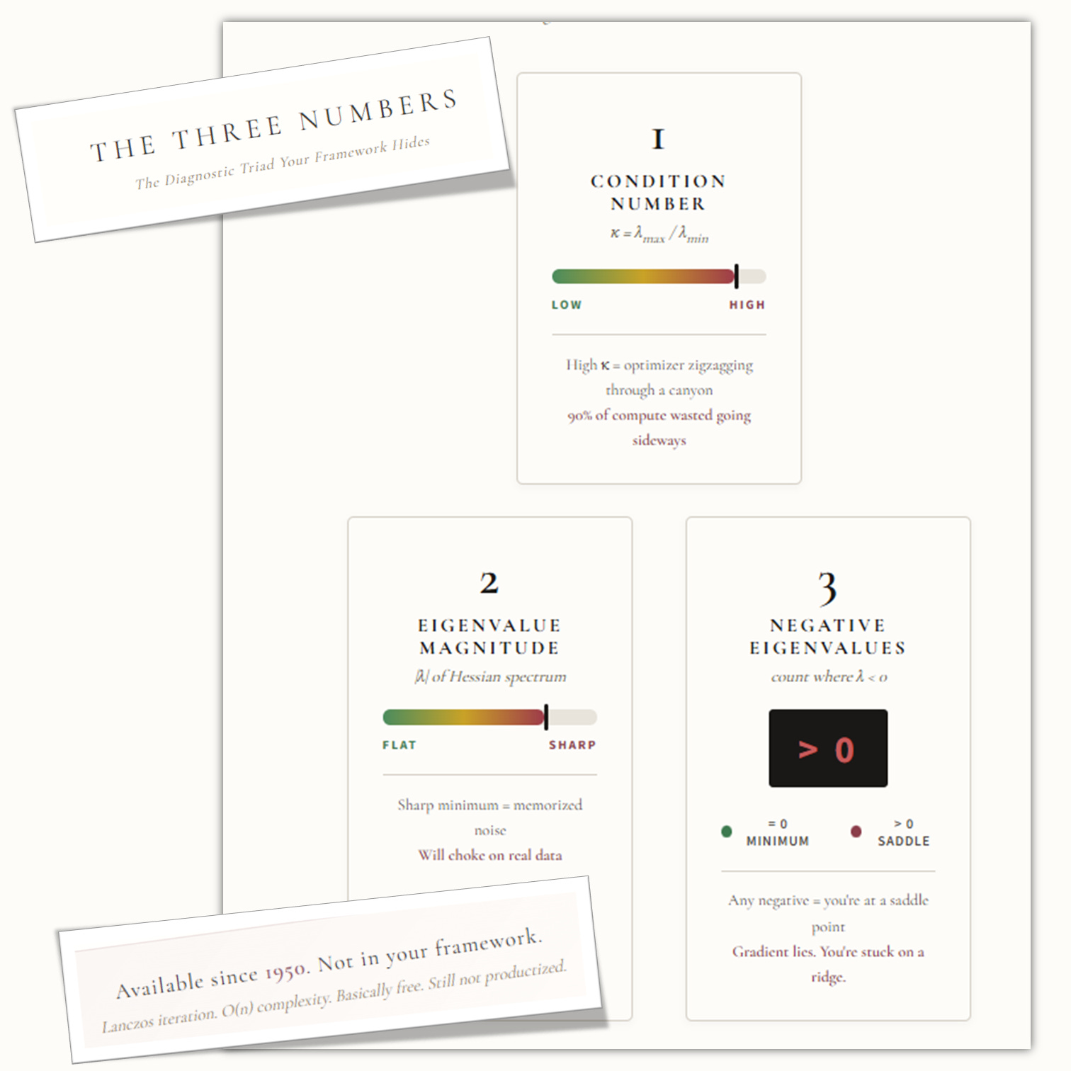
The Three Numbers Everyone Ignores

Nobody tells you about them. Not your framework. Not your coursework. Not the documentation, though they predict whether your training will work or blow up in your face. Whether inference will be stable or hallucinatory. Whether your minimum is real or a trap.

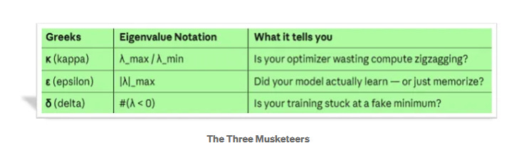
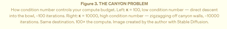
1. Condition number κ (λ_max / λ_min): Is your optimizer wasting compute zig-zagging? This number measures how “stretched” your loss landscape is. A high κ means canyon. You’re burning 90% of your compute going sideways instead of down (direction towards the error minimum)

2. Eigenvalue magnitude ε (|λ|_max): Did your model actually learn — or just memorize? Read on, and you’ll find a cute GIF below that explains it better than a whole series of equations..

3. Negative eigenvalue count δ (#λ < 0):
You might be convinced that the gradient from your AI framework is enough to finish training your shiny new network. That’s what you were told: the gradient says “we’re done, nowhere to go” because the slope is flat in every direction you’re measuring.

But what if your training is stuck at a fake minimum?
That’s what this killer δ number is for. As a preview:

• When δ = 0, you’re at a true minimum — a valley floor.

• When δ > 0, you’re on a mountain ridge.

Further below you’ll see an animated graphic that will clarify the questions you’re probably asking yourself right now.

And Yet — Believe It or Not — This Is Old Math

This math has existed since 1950. Before anyone had dreamed of a neural network.

Seventy-five years of mathematicians screaming into the void.

And still — right now, today, as you read this — not in PyTorch. Not in TensorFlow. Not in JAX. Not in Keras. Not in any standard training pipeline burning millions of dollars.

Three numbers that would tell you everything. Hidden in plain sight.

The biggest AI labs in the world? They’re watching loss curves. Crossing fingers. And calling it engineering.

OpenAI ignores them. Google skips them. Anthropic doesn’t even know they exist. Nobody checks.

Let it sink in. But keep reading, you haven’t seen the best part yet.

The Three Numbers Everyone Misses

So you’ve met κ, ε, and δ. Three numbers that predict everything. Three numbers that have existed since your grandparents were young.

Now ask yourself: where are they?

Not on your screen. Not in your logs. Not anywhere in the trillion-dollar AI industry.

Those three numbers aren’t theory. They’re a diagnostic panel that should exist… but doesn’t.

Instead, here’s what the most popular AI frameworks — PyTorch, TensorFlow, JAX, Keras — actually give you:

• Loss value ✓

• Gradient direction ✓

• Learning rate ✓

That’s it. That’s the whole dashboard.

Three numbers — but not the right three. Not κ (condition number). Not ε (eigenvalue magnitude). Not δ (negative eigenvalue count).

And it’s not just your framework. OpenAI’s internal tools? Same blind spot. Google’s infrastructure? Same gap. Anthropic’s training pipeline? Same missing panel. The entire industry is flying the same broken instrument cluster.

Training AI today is like flying a 747 with a speedometer, a compass, and vibes.

The loss is going down. Great — that means the error is going down, training looks good.

But why is it going down? Is the model finding a real solution, or just memorizing noise and digging itself into a hole it’ll never escape?

The eigenvalues would tell you. Your favorite AI framework’s dashboard won’t.

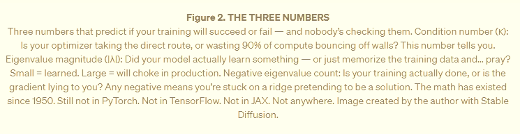
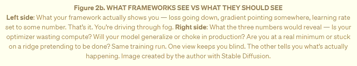
Figure 2b makes this obvious:

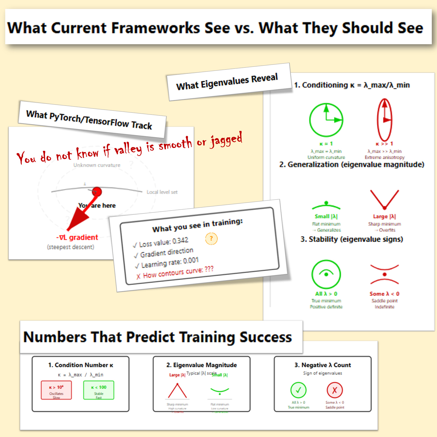
Where those three numbers come from

They live inside something called the Hessian: the second derivative matrix of your loss function. It encodes the complete curvature of your loss landscape. Every canyon, every ridge, every flat plateau. It’s all there.

And here’s the absurd part: the Hessian is fully computable. It’s sitting right there, screaming diagnostic data, and nobody’s looking at it.

Here’s how it works:

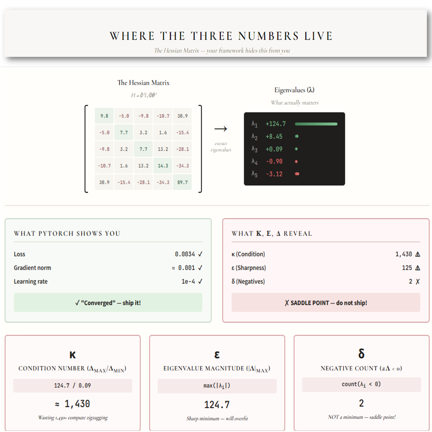
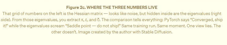
Look at the two boxes in the middle of the figure. On the left: what PyTorch shows you. Loss looks good. Gradient near zero. Learning rate set. Green light. Ship it.

On the right: what κ, ε, and δ reveal. Condition number through the roof. Sharpness off the charts. Two negative eigenvalues. You’re not at a minimum: you’re stuck at a saddle point pretending to be done. 💀

Same numbers. Same moment. Opposite conclusions.

OpenAI doesn’t compute this. Google doesn’t compute this.

Nobody running a several-hundred-thousand-bucks-a-month GPU cluster is checking eigenvalues.

They’re watching loss curves and you guessed right… praying!

But the Hessian is Too Heavy!

This is where someone from Google raises their hand.

The Hessian is n×n. For a billion-parameter model, that’s a billion times a billion. You can’t compute that. It’s mathematically insane !

Correct. And completely irrelevant.

You don’t need the full matrix. You never did.

A Hungarian physicist named Cornelius Lanczos figured this out in 1950 — back when “computer” meant a room full of vacuum tubes and an obsessive cross-fingering. His method extracts the dominant eigenvalues using iterative matrix-vector products. Complexity: O(n) per iteration. Basically free compared to a single forward pass.

Seventy-five years of progress since then? We now have Hutchinson’s trace estimator, stochastic Lanczos quadrature, randomized SVD. You can get spectral density estimates, top-k eigenvalues, condition number bounds — all at negligible computational cost.

Tools like PyHessian already prove this works at ImageNet scale. Today. Right now.

So why isn’t this in PyTorch? Why isn’t it in TensorFlow? Why isn’t it in JAX?

Because the people who understand spectral theory are in math departments writing papers nobody reads. The people building frameworks are shipping features that look good in demos. And the people training models are too busy babysitting loss curves to ask why they’re babysitting loss curves.

The math exists. The engineering exists. The will to connect them? Apparently not.

Seventy-five years. Still waiting…

What These Numbers Actually Tell You

Let’s make this practical, concrete, and — above all — visual, so you can build the right mathematical intuitions.

The Condition Number Disaster

The condition number κ (kappa) = λ_max / λ_min controls how hard your optimization problem actually is.

Here’s what nobody tells you: gradient descent convergence scales as (κ-1)/(κ+1) per iteration.

Translation:

• κ = 100? Roughly 100 iterations to cut your error in half.

• κ = 10000? Roughly 10k iterations for the same progress.

And κ = 10000 is common in practice. Not pathological. Not rare. Tuesday.

So what does high κ feel like?

Imagine rolling a marble down a valley. Nice round bowl? Marble rolls straight to the bottom. Done.

But high κ means your valley is a razor-thin slot canyon: walls a mile high, floor barely visible. Your marble doesn’t roll down. It pinballs off the walls. Left. Right. Left. Right. Burning energy going sideways instead of down.

That’s your gradient. Pointing exactly where calculus says: steepest downhill. Problem is, “steepest downhill” aims at the canyon walls, not down the floor toward the solution.

Those training runs that plateau for hours? Loss stuck at 0.0847, then 0.0846, then 0.0847 again? You tweak the learning rate. Nothing. You sacrifice a rubber duck to the ML gods🚮 . Nothing.

That’s high κ.

Your optimizer isn’t broken. It’s doing exactly what you asked. What you asked is just geometrically insane.

You’re burning compute fighting geometry your framework refuses to acknowledge exists.

The fix?

Preconditioning. Second-order methods. Adaptive optimizers that implicitly estimate curvature. The math exists. It’s been in textbooks since the 1960s.

But first, you’d need to know κ is the problem.

Your dashboard won’t tell you. So you’ll never ask. And your compute bill keeps climbing.

The figure below shows exactly what’s happening. Same starting point. Same destination. One path takes ~100 iterations. The other takes ~10000 — zigzagging off canyon walls while your GPU burns money.

Sharp vs. Flat: The Generalization Prophecy

Now let’s talk about ε (epsilon) — the eigenvalue magnitude |λ|_max.

This number answers the question every ML engineer secretly dreads: Did your model actually learn anything, or did it just memorize the test?

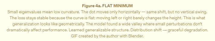
Picture your loss landscape as terrain. A flat minimum is a wide valley — you can wander around and the elevation barely changes. A sharp minimum is a knife-edge ridge — one wrong step and you’re tumbling into the abyss.

Small ε = flat minimum = good news.

When ε is small, your model found that wide valley. Production data comes in slightly different from training data: users type weird things, lighting changes, accents vary, and your model shrugs. Close enough. I got this.

That’s generalization. That’s what you’re paying for.

The GIF below shows what this looks like geometrically:

Now flip the script.

What happens when ε is huge? When your eigenvalues are screaming large numbers?

Well, when ε is large, your model has squeezed itself into a tiny, sharp crevice. Training loss looks perfect. Validation is “best run ever.”

Then real data arrives. Slightly different wording. Slightly different images. Slightly different anything.

And the model doesn’t perform a bit worse. It blows up:

• Confidence scores go crazy

• Predictions turn random

• Your alert-log system explodes at 2 AM. 💀

That’s a sharp minimum in action. The walls are so steep that the tiniest shift sends the loss rocketing. Your model wasn’t robust. It was brittle and faking it.

The GIF below shows the difference. Same horizontal shift. Wildly different outcomes.

As you see this is not philosophy. This is geometry you can measure.

Your model that crushed the benchmark and died in production? It found a sharp minimum. The eigenvalues would have told you… but nobody checked.

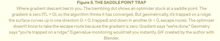
Saddle Points: The Silent Killer

Now for δ (delta) — the negative eigenvalue count, #(λ < 0). This one’s sneaky. This one lies to your face.

Your gradient hits zero.
Your loss curve goes flat.
Your framework prints: “converged.”
You relax.

But you’re not at an error minimum.
You’re at a saddle point ! 💀

A mountain pass where the terrain curves up in some directions and down in others.

But you might say: PyTorch shows my gradient is zero — shouldn’t that mean the optimization is done?
No, dear reader. No. It only means you’re balanced on a ridge, not that you’ve reached anything useful.

How common are saddle points?

Let’s do the math.

At any critical point, you can think of each eigenvalue as having a coin-flip chance of being positive or negative. For a true minimum, you need all of them positive. The rough probability? One-half raised to the power of your parameter dimension.

For a million parameters, that’s 1/ 2^(10⁶).

You have better odds of winning the lottery while being struck by lightning while a shark bites your leg. In high dimensions, almost every critical point is effectively a saddle. True minima are statistical miracles.

The good news: most saddle points are unstable. SGD’s inherent noise usually kicks you off eventually.

The bad news: “eventually” might be three weeks of wasted compute. Degenerate saddles — where eigenvalues hover near zero — create plateaus where the gradient whispers instead of speaks. Loss goes nowhere. You’re stuck, but you don’t know if you’re stuck or just slow.

δ > 0 would tell you instantly. One number. Saddle or not. But your framework doesn’t compute it.

The GIF below shows what this trap looks like:

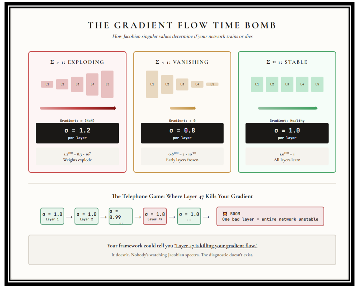
The Gradient Flow Time Bomb

Oh, you thought we were done? It gets worse.

Your neural network isn’t one function. It’s a chain of functions — layer after layer after layer. And gradients have to flow backward through every single one during training. Like a game of telephone, except each person might whisper too quietly or scream too loud.

Each layer has a Jacobian matrix — the matrix of partial derivatives that governs how signals propagate. The singular values of these Jacobians determine whether your gradients survive the journey or die along the way.

Singular values > 1: The gradient gets amplified at each layer. By the time it reaches the early layers, it’s not a gradient anymore — it’s a bomb. Exploding gradients. Your weights go to infinity. Training crashes. NaN city.

Singular values < 1: The opposite disaster. The gradient gets squashed at each layer. By the time it reaches the early layers, it’s a rounding error. Vanishing gradients. Your early layers stop learning. They’re frozen while the rest of the network pretends to train.

Singular values ≈ 1: Goldilocks zone. Gradients flow cleanly from end to end. Every layer learns. This is why orthogonal initialization works. This is why spectral normalization exists.

But here’s the thing: these techniques were discovered by accident and applied as band-aids. Nobody monitors Jacobian spectra during training. Nobody watches the singular values drift. The diagnostic that would tell you: Layer 47 is about to kill your gradient flow 😁, simply doesn’t exist in any commercial framework.

Your network could be bleeding out internally, and the dashboard shows nothing.

See it for yourself:

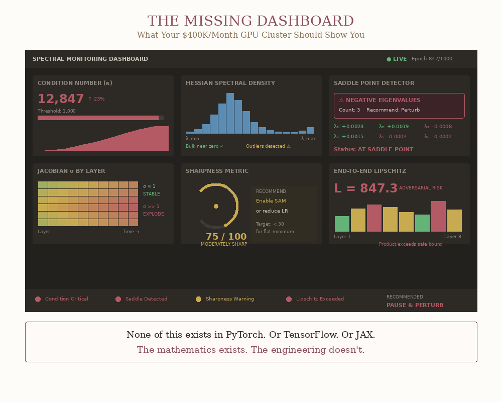
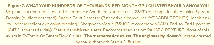
And Here You Go: The Real Dashboard Your AI Framework Is Missing

This is the dashboard a serious AI framework should show you.

A mathematically literate training loop would compute lightweight spectral diagnostics at checkpoints and act on them:

• Hessian condition number exceeds a threshold → switch to a preconditioned method.

• Jacobian singular values drift away from 1 → apply spectral normalization.

• Negative eigenvalues appear → you’re at a saddle, perturb to escape.

Right now, no commercially available AI framework gives you these basic eigenvalue predictors. Instead, you’re hand-tuning learning rates and hoping…

Why Nobody Fixed This

Three reasons:

Scaling obscures mathematical sins. When throwing more compute at the problem works, nobody questions the foundations. This is temporary. Scaling laws plateau. When they do, the industry will suddenly need mathematics it never bothered to learn.

Disciplinary silos. The people who understand spectral theory work in applied math departments solving inverse problems. The people building AI frameworks took optimization and statistics. The Venn diagram overlap is nearly empty.

Abstraction debt. Implementing proper spectral monitoring requires infrastructure nobody wants to build. Everyone would benefit. Nobody wants to pay.

The Bill Comes Due

Here’s what’s missing in every production framework:

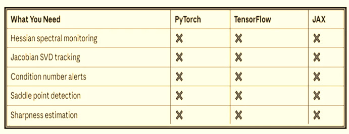
The industry has invested $100 billion in scaling AI.

The mathematical foundations remain incomplete.

Every unexplained training failure, every generalization anomaly, every model that worked in the lab and died in production — these are symptoms of mathematical pathologies that your tools cannot diagnose.

What You Can Do Now to go even beyond those big AI companies ?

Start here:

1. Learn what Hessian eigenvalues mean for your specific architecture

2. Monitor condition numbers during training — even crude estimates help

3. Check for sharpness before you ship — PyHessian exists, use it

4. Question everything when loss plateaus — you might be at a saddle, not a minimum

The math exists. It’s been waiting since 1950.

The only question is whether you’ll learn it before your next production failure teaches you the hard way.