Why AI Isn’t Flat: The Hidden Curvature

Holonomy, Jacobians, and Curvature Emerging from Flat Space

Where Flat AI Bends Space...

TL;DR — Why AI Isn’t Flat


1. Curvature emerges automatically in any nonlinear DAG.

\(\begin{array}{l} \text{Even if your model lives in plain } \mathbb{R}^n, \text{ a nonlinear DAG plus autodiff defines} \\ \text{Jacobian blocks } \Gamma_{ij} = dY_i/dX_i \text{ between sites. Composing them around tiny} \\ \text{loops } H_{ijk} = \Gamma_{ki} \Gamma_{jk} \Gamma_{ij} \text{ almost never gives the identity. That path-} \\ \text{dependence of infinitesimal transport } \textit{is} \text{ curvature. You get geometry "for free"} \\ \text{as soon as you stack nonlinear layers.} \end{array}\)

2. Holonomy is the right diagnostic for model “twist zones”.

\(\begin{array}{l} \text{Curvature is not a scalar you sprinkle on a layer; it's the failure of transport to be} \\ \text{path-independent. Holonomy } H_{ijk} \text{ measures exactly that: nudge a vector at } i, \\ \text{move it through } j \text{ and } k, \text{ and bring it back. Where } \|H_{ijk} - I\| \text{ is large, the model} \\ \text{is twisting, shearing, and reinterpreting signals. Those are your } \textbf{twist zones}\text{---} \\ \text{regions of complex, context-sensitive behaviour.} \end{array}\)

3. Euclidean embeddings are an illusion.

We store vectors in Euclidean tensors, but the network never treats them as living in a globally flat space. Because transport is curved, the “meaning” of a direction in embedding space depends on where you are and how you got there. The coordinates are Euclidean; the effective geometry induced by the Jacobians is not. “Flat embeddings” are a convenient lie.

4. AI needs explicit geometry (toroidal memory, hyperbolic hierarchy).

If geometry is unavoidable, we might as well choose the right one. Toroidal memory eliminates artificial edges and wrap-around glitches; hyperbolic spaces encode trees and hierarchies naturally. Making these structures explicit lets memory, recall, and abstraction live in geometries that actually match the tasks, instead of in accidental curvature produced by random stacks of layers.

5. A geometric AI OS fixes the accident-geometry problem.

Today’s AI discovers curvature by accident: opaque, emergent, and hard to control. A geometric OS flips the story. You design the state spaces (toroidal / hyperbolic), you specify the connection via duals and jets, and you treat Γ and H as first-class, auditable objects—not hidden side-effects of backprop. Curvature stops being a bug you diagnose after training and becomes an operating principle you engineer from the start.

1. Holonomy Toolkit – Fibers, Jacobians, Transport Maps, and Loops

Let’s start with an easy, practical definition of holonomy:

Holonomy is what the network does to a tiny perturbation when you send it around a loop of sites and bring it back.

Want it a bit more concrete? Here you go:

Holonomy is what you get when you move a vector around a closed loop and see how much it has changed when you return to the starting point.

In geometric language, you have a space with a connection (rules for transporting vectors along paths). You pick a point, take a vector in its fiber, and parallel–transport that vector along a loop that begins and ends at the same point.

The resulting linear map — comparing the final vector to the original one — is, formally, the holonomy of that loop:

\(\begin{array}{l} H_\gamma : V_i \to V_i \\ \\ \text{is called the } \textbf{holonomy} \text{ of that loop } \gamma. \\ \\ \text{• If } H_\gamma \text{ is the identity for every loop, the space is "flat": transport around} \\ \quad \text{any loop brings every vector back unchanged.} \\ \text{• If some loop has } H_\gamma \neq I, \text{ then the space has } \textbf{curvature}\text{: going around} \\ \quad \text{that loop twists or rotates vectors in a detectable way.} \end{array}\)

For a more detailed depiction of how holonomy theory was created over several generations of mathematicians, I strongly recommend reading my other article here.


And now the ingredients of the holonomy recipe:

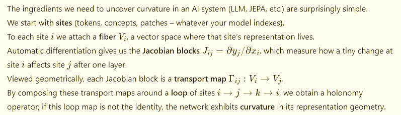
2. The Holonomy in Action:

We begin with three sites i,j,k inside a single neural network layer.

\(\begin{array}{l} \text{At each site we have an underlying Euclidean fiber } V_i \cong \mathbb{R}^d. \\ \\ \text{Given a differentiable layer } F : \mathbb{R}^{n \times d} \to \mathbb{R}^{n \times d}, \text{ we denote} \\ \\ \Gamma_{ij} = \frac{\partial Y_j}{\partial X_i} \end{array}\)

the Jacobian block mapping infinitesimal variations at i to infinitesimal effects at j. These blocks exist for any modern deep-learning layer, because AD computes them implicitly via JVP/VJP.

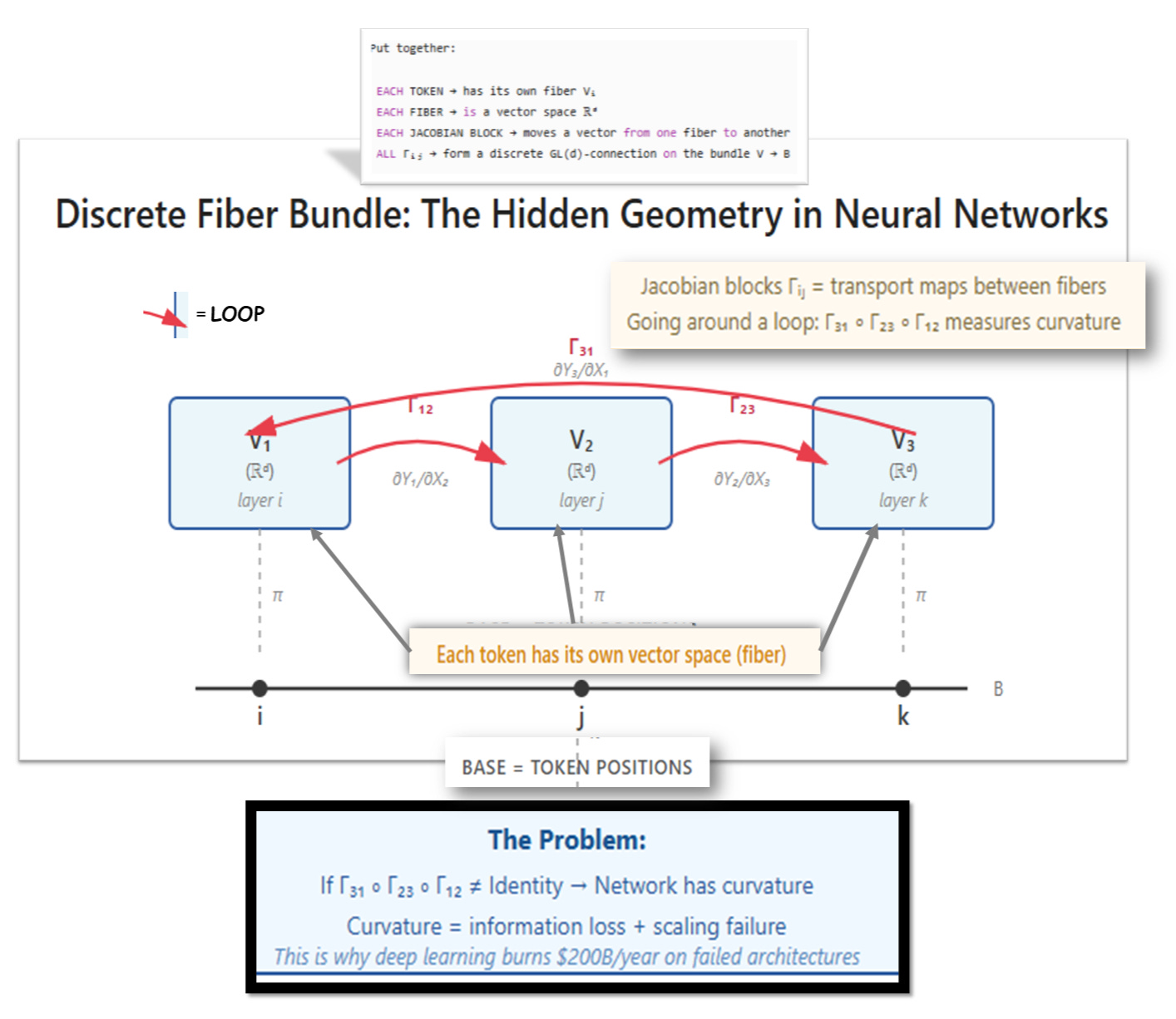
We then form the holonomy operator along the discrete loop i→j→k→i:

\(H_{ijk} = \Gamma_{ki} \, \Gamma_{jk} \, \Gamma_{ij}.\)

If the induced connection on the discrete bundle is flat, the holonomy on every such small loop is trivial:

\(H_{ijk} = I_d.\)

\(\begin{array}{l} \text{where } I_d \text{ is the identity operator on the fiber } V_i \cong \mathbb{R}^d \text{ (it sends every} \\ \text{tiny vector at site } i \text{ back to itself)} \end{array}\)

In general nonlinear architectures—attention, LayerNorm, GELU, gating—the Jacobian blocks do not commute. Algebraically this means, for typical sites,

\(\Gamma_{jk} \Gamma_{ij} \neq \Gamma_{ij} \Gamma_{jk}\)

so the effect of applying one transport and then the other depends on the order. This non-commutativity by itself is an operator property; its geometric consequence is path-dependence: moving a perturbation through “path 1 then path 2” is not the same as “path 2 then path 1”.

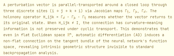
For our specific triangle i→j→k→i, that path-dependence shows up as non-trivial holonomy: there exists some perturbation v ∈ Vi​ such that:

\(H_{ijk} v \neq v\)

So the loop returns to the same site i but not to the same vector. In short,

\(H_{ijk} \neq I_d.\)

Which is exactly the discrete signature of curvature on that loop.

This phenomenon arises even though:

1. The underlying state space is Euclidean.

2. The architecture is a directed acyclic graph.

3. No explicit manifold structure is specified.

Curvature is therefore emergent, not designed. It is induced purely by the nonlinearity of the DAG and the resulting non-integrability of the local transport operators.

It happens even though your model lives in flat Rⁿ and has no cycles. Because the model’s nonlinearities bend the transport rules even when the coordinates are straight.

That’s the paradox the plot above reveals.

3. Why the Loop Exists in the Math but Not in the Architecture

Formally, the architecture is a DAG.
There are no computational cycles.

The Tiny Loop That Reveals AI’s Geometry.

Yet the holonomy loop exists because differentiation produces linear transport operators that you can compose arbitrarily, independent of the forward DAG.

Let’s formalize:

For a fixed layer FFF, define its Jacobian as a block matrix:

\(J = [\Gamma_{i,i-1}]_{i=1}^n\)

This matrix defines a connection on the discrete set of sites.
The network architecture restricts which forward edges exist, but the Jacobian-level transport is independent of acyclic structure: it exists because AD defines Γij for all relevant pairs.

A loop in this connection is therefore a loop in operator space, not in the data-flow graph.
Holonomy is computed over compositions of differential maps, not over actual physical cycles of computation.

The result:
even a DAG can induce a connection with non-zero curvature.

4. Why Curvature Emerges Automatically

Mathematically:

Curvature appears whenever the transport operators fail to satisfy the discrete integrability condition:

\(\Gamma_{ki} \Gamma_{jk} \Gamma_{ij} = I.\)

In nonlinear DAGs, this fails generically because:

• nonlinear activations distort tangent directions,

• attention weights depend on content and therefore break symmetry,

• LayerNorm rescales each site differently,

• residual mixing causes non-commutativity of Jacobian blocks,

• depth compounds these non-integrabilities.

Thus curvature is not exceptional.
It is structurally expected.

As soon as each site interacts with others in a state-dependent, nonlinear manner, path-dependence becomes unavoidable.

5.Euclidean Embeddings Are an Illusion

Mathematically:

Even if the representation space is R^d, the connection induced by the Jacobians defines a non-Euclidean geometry on the bundle of site-wise fibers.

Thus the “geometry” relevant for signal transport is not the coordinate geometry of the ambient space, but the connection geometry induced by the architecture.

The embedding vectors sit in a Euclidean vector space,
but the model’s transformations define a geometry that is almost never Euclidean.

6. Why AI Needs Explicit Geometry (How Our AI-Operating System Fixes This)

Because curvature is emergent, uncontrolled, and opaque, it produces:

• semantic drift across layers,

• unstable gradients,

• inconsistent meaning of directions,

• poor memory retention,

• interpretability breakdowns.

A geometric OS solves this by:

• using toroidal memory for stable, boundaryless recall,

• using hyperbolic representation spaces for hierarchy and abstraction,

• defining a controlled connection via duals and jets,

• enforcing implementation-independent transport.

SUMMING UP…

Curvature stops being a side-effect and becomes an engineered property.

Right now, your model invents its geometry by accident.

Sometimes it works.
Sometimes it collapses.

A geometric OS says:

“No more accidental geometry.
We choose the curvature, we choose the memory topology,
and we choose how information moves.”

And suddenly AI becomes predictable, auditable, and mathematically grounded.